11 Statistical learning

Prerequisites

This chapter assumes proficiency with geographic data analysis, for example gained by studying the contents and working-through the exercises in Chapters 2 to 6. A familiarity with generalized linear models (GLM) and machine learning is highly recommended (for example from A. Zuur et al. 2009; James et al. 2013).

The chapter uses the following packages:⁶⁶

library(sf)
library(raster)
library(dplyr)

library(mlr)
library(parallelMap)

Required data will be attached in due course.

11.1 Introduction

Statistical learning is concerned with the use of statistical and computational models for identifying patterns in data and predicting from these patterns. Due to its origins, statistical learning is one of R’s great strengths (see Section 1.3).⁶⁷ Statistical learning combines methods from statistics and machine learning and its methods can be categorized into supervised and unsupervised techniques. Both are increasingly used in disciplines ranging from physics, biology and ecology to geography and economics (James et al. 2013).

This chapter focuses on supervised techniques in which there is a training dataset, as opposed to unsupervised techniques such as clustering. Response variables can be binary (such as landslide occurrence), categorical (land use), integer (species richness count) or numeric (soil acidity measured in pH). Supervised techniques model the relationship between such responses — which are known for a sample of observations — and one or more predictors.

The primary aim of much machine learning research is to make good predictions, as opposed to statistical/Bayesian inference, which is good at helping to understand underlying mechanisms and uncertainties in the data (see Krainski et al. 2018). Machine learning thrives in the age of ‘big data’ because its methods make few assumptions about input variables and can handle huge datasets. Machine learning is conducive to tasks such as the prediction of future customer behavior, recommendation services (music, movies, what to buy next), face recognition, autonomous driving, text classification and predictive maintenance (infrastructure, industry).

This chapter is based on a case study: the (spatial) prediction of landslides. This application links to the applied nature of geocomputation, defined in Chapter 1, and illustrates how machine learning borrows from the field of statistics when the sole aim is prediction. Therefore, this chapter first introduces modeling and cross-validation concepts with the help of a Generalized Linear Model (A. Zuur et al. 2009). Building on this, the chapter implements a more typical machine learning algorithm, namely a Support Vector Machine (SVM). The models’ predictive performance will be assessed using spatial cross-validation (CV), which accounts for the fact that geographic data is special.

CV determines a model’s ability to generalize to new data, by splitting a dataset (repeatedly) into training and test sets. It uses the training data to fit the model, and checks its performance when predicting against the test data. CV helps to detect overfitting since models that predict the training data too closely (noise) will tend to perform poorly on the test data.

Randomly splitting spatial data can lead to training points that are neighbors in space with test points. Due to spatial autocorrelation, test and training datasets would not be independent in this scenario, with the consequence that CV fails to detect a possible overfitting. Spatial CV alleviates this problem and is the central theme in this chapter.

11.2 Case study: Landslide susceptibility

This case study is based on a dataset of landslide locations in Southern Ecuador, illustrated in Figure 11.1 and described in detail in Muenchow, Brenning, and Richter (2012). A subset of the dataset used in that paper is provided in the RSAGA package, which can be loaded as follows:

data("landslides", package = "RSAGA")

This should load three objects: a data.frame named landslides, a list named dem, and an sf object named study_area. landslides contains a factor column lslpts where TRUE corresponds to an observed landslide ‘initiation point,’ with the coordinates stored in columns x and y.⁶⁸

There are 175 landslide points and 1360 non-landslide, as shown by summary(landslides). The 1360 non-landslide points were sampled randomly from the study area, with the restriction that they must fall outside a small buffer around the landslide polygons.

To make the number of landslide and non-landslide points balanced, let us sample 175 from the 1360 non-landslide points.⁶⁹

# select non-landslide points
non_pts = filter(landslides, lslpts == FALSE)
# select landslide points
lsl_pts = filter(landslides, lslpts == TRUE)
# randomly select 175 non-landslide points
set.seed(11042018)
non_pts_sub = sample_n(non_pts, size = nrow(lsl_pts))
# create smaller landslide dataset (lsl)
lsl = bind_rows(non_pts_sub, lsl_pts)

dem is a digital elevation model consisting of two elements: dem$header, a list which represents a raster ‘header’ (see Section 2.3), and dem$data, a matrix with the altitude of each pixel. dem can be converted into a raster object with:

dem = raster(
  dem$data, 
  crs = dem$header$proj4string,
  xmn = dem$header$xllcorner, 
  xmx = dem$header$xllcorner + dem$header$ncols * dem$header$cellsize,
  ymn = dem$header$yllcorner,
  ymx = dem$header$yllcorner + dem$header$nrows * dem$header$cellsize
  )

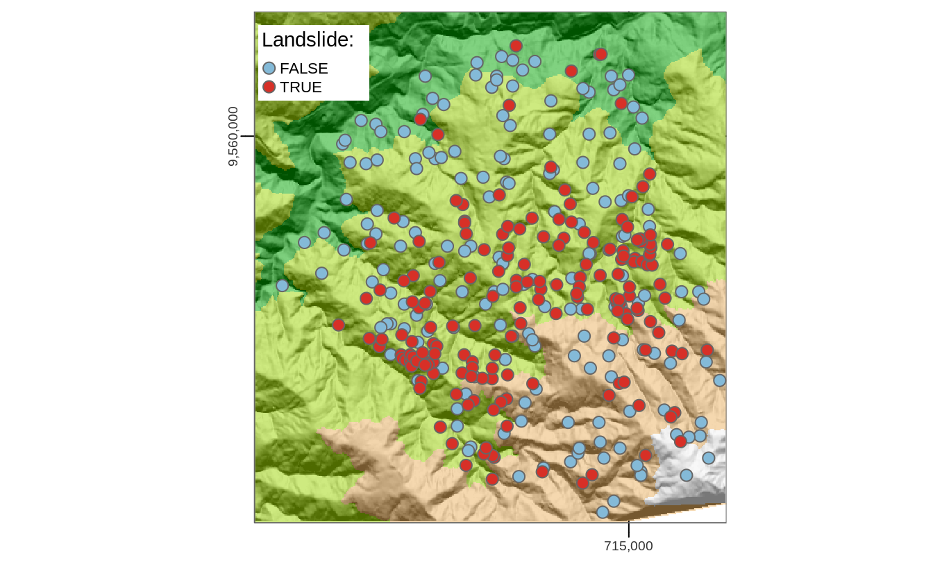
FIGURE 11.1: Landslide initiation points (red) and points unaffected by landsliding (blue) in Southern Ecuador.

To model landslide susceptibility, we need some predictors. Terrain attributes are frequently associated with landsliding (Muenchow, Brenning, and Richter 2012), and these can be computed from the digital elevation model (dem) using R-GIS bridges (see Chapter 9). We leave it as an exercise to the reader to compute the following terrain attribute rasters and extract the corresponding values to our landslide/non-landslide data frame (see exercises; we also provide the resulting data frame via the spDataLarge package, see further below):

slope: slope angle (°).
cplan: plan curvature (rad m⁻¹) expressing the convergence or divergence of a slope and thus water flow.
cprof: profile curvature (rad m^-1) as a measure of flow acceleration, also known as downslope change in slope angle.
elev: elevation (m a.s.l.) as the representation of different altitudinal zones of vegetation and precipitation in the study area.
log10_carea: the decadic logarithm of the catchment area (log10 m²) representing the amount of water flowing towards a location.

Data containing the landslide points, with the corresponding terrain attributes, is provided in the spDataLarge package, along with the terrain attribute raster stack from which the values were extracted. Hence, if you have not computed the predictors yourself, attach the corresponding data before running the code of the remaining chapter:

# attach landslide points with terrain attributes
data("lsl", package = "spDataLarge")
# attach terrain attribute raster stack
data("ta", package = "spDataLarge")

The first three rows of lsl, rounded to two significant digits, can be found in Table 11.1.

TABLE 11.1: Structure of the lsl dataset.
x	y	lslpts	slope	cplan	cprof	elev	log10_carea
715078	9558647	FALSE	37	0.021	0.009	2500	2.6
713748	9558047	FALSE	42	-0.024	0.007	2500	3.1
712508	9558887	FALSE	20	0.039	0.015	2100	2.3

11.3 Conventional modeling approach in R

Before introducing the mlr package, an umbrella-package providing a unified interface to dozens of learning algorithms (Section 11.5), it is worth taking a look at the conventional modeling interface in R. This introduction to supervised statistical learning provides the basis for doing spatial CV, and contributes to a better grasp on the mlr approach presented subsequently.

Supervised learning involves predicting a response variable as a function of predictors (Section 11.4). In R, modeling functions are usually specified using formulas (see ?formula and the detailed Formulas in R Tutorial for details of R formulas). The following command specifies and runs a generalized linear model:

fit = glm(lslpts ~ slope + cplan + cprof + elev + log10_carea,
          family = binomial(),
          data = lsl)

It is worth understanding each of the three input arguments:

A formula, which specifies landslide occurrence (lslpts) as a function of the predictors
A family, which specifies the type of model, in this case binomial because the response is binary (see ?family)
The data frame which contains the response and the predictors

The results of this model can be printed as follows (summary(fit) provides a more detailed account of the results):

class(fit)
#> [1] "glm" "lm"
fit
#> 
#> Call:  glm(formula = lslpts ~ slope + cplan + cprof + elev + log10_carea, 
#>     family = binomial(), data = lsl)
#> 
#> Coefficients:
#> (Intercept)        slope        cplan        cprof         elev  log10_carea  
#>    1.97e+00     9.30e-02    -2.57e+01    -1.43e+01     2.41e-05    -2.12e+00  
#> 
#> Degrees of Freedom: 349 Total (i.e. Null);  344 Residual
#> Null Deviance:       485 
#> Residual Deviance: 361   AIC: 373

The model object fit, of class glm, contains the coefficients defining the fitted relationship between response and predictors. It can also be used for prediction. This is done with the generic predict() method, which in this case calls the function predict.glm(). Setting type to response returns the predicted probabilities (of landslide occurrence) for each observation in lsl, as illustrated below (see ?predict.glm):

pred_glm = predict(object = fit, type = "response")
head(pred_glm)
#>      1      2      3      4      5      6 
#> 0.3327 0.4755 0.0995 0.1480 0.3486 0.6766

Spatial predictions can be made by applying the coefficients to the predictor rasters. This can be done manually or with raster::predict(). In addition to a model object (fit), this function also expects a raster stack with the predictors named as in the model’s input data frame (Figure 11.2).

# making the prediction
pred = raster::predict(ta, model = fit, type = "response")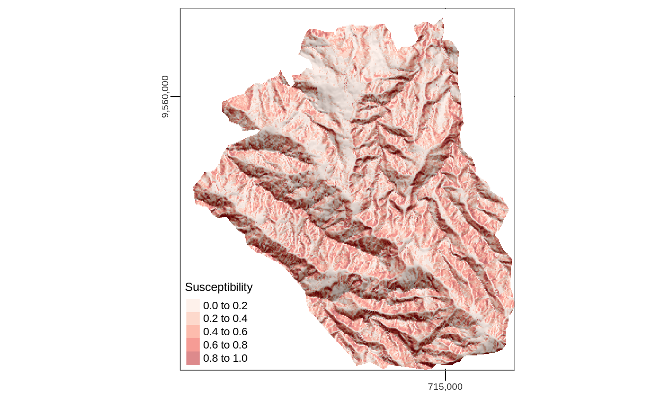

FIGURE 11.2: Spatial prediction of landslide susceptibility using a GLM.

Here, when making predictions we neglect spatial autocorrelation since we assume that on average the predictive accuracy remains the same with or without spatial autocorrelation structures. However, it is possible to include spatial autocorrelation structures into models (A. Zuur et al. 2009; Blangiardo and Cameletti 2015; A. F. Zuur et al. 2017) as well as into predictions (kriging approaches, see, e.g., Goovaerts 1997; Hengl 2007; R. Bivand, Pebesma, and Gómez-Rubio 2013). This is, however, beyond the scope of this book.

Spatial prediction maps are one very important outcome of a model. Even more important is how good the underlying model is at making them since a prediction map is useless if the model’s predictive performance is bad. The most popular measure to assess the predictive performance of a binomial model is the Area Under the Receiver Operator Characteristic Curve (AUROC). This is a value between 0.5 and 1.0, with 0.5 indicating a model that is no better than random and 1.0 indicating perfect prediction of the two classes. Thus, the higher the AUROC, the better the model’s predictive power. The following code chunk computes the AUROC value of the model with roc(), which takes the response and the predicted values as inputs. auc() returns the area under the curve.

pROC::auc(pROC::roc(lsl$lslpts, fitted(fit)))
#> Area under the curve: 0.826

An AUROC value of 0.83 represents a good fit. However, this is an overoptimistic estimation since we have computed it on the complete dataset. To derive a biased-reduced assessment, we have to use cross-validation and in the case of spatial data should make use of spatial CV.

11.4 Introduction to (spatial) cross-validation

Cross-validation belongs to the family of resampling methods (James et al. 2013). The basic idea is to split (repeatedly) a dataset into training and test sets whereby the training data is used to fit a model which then is applied to the test set. Comparing the predicted values with the known response values from the test set (using a performance measure such as the AUROC in the binomial case) gives a bias-reduced assessment of the model’s capability to generalize the learned relationship to independent data. For example, a 100-repeated 5-fold cross-validation means to randomly split the data into five partitions (folds) with each fold being used once as a test set (see upper row of Figure 11.3). This guarantees that each observation is used once in one of the test sets, and requires the fitting of five models. Subsequently, this procedure is repeated 100 times. Of course, the data splitting will differ in each repetition. Overall, this sums up to 500 models, whereas the mean performance measure (AUROC) of all models is the model’s overall predictive power.

However, geographic data is special. As we will see in Chapter 12, the ‘first law’ of geography states that points close to each other are, generally, more similar than points further away (Miller 2004). This means these points are not statistically independent because training and test points in conventional CV are often too close to each other (see first row of Figure 11.3). ‘Training’ observations near the ‘test’ observations can provide a kind of ‘sneak preview’: information that should be unavailable to the training dataset. To alleviate this problem ‘spatial partitioning’ is used to split the observations into spatially disjointed subsets (using the observations’ coordinates in a k-means clustering; Brenning (2012b); second row of Figure 11.3). This partitioning strategy is the only difference between spatial and conventional CV. As a result, spatial CV leads to a bias-reduced assessment of a model’s predictive performance, and hence helps to avoid overfitting.

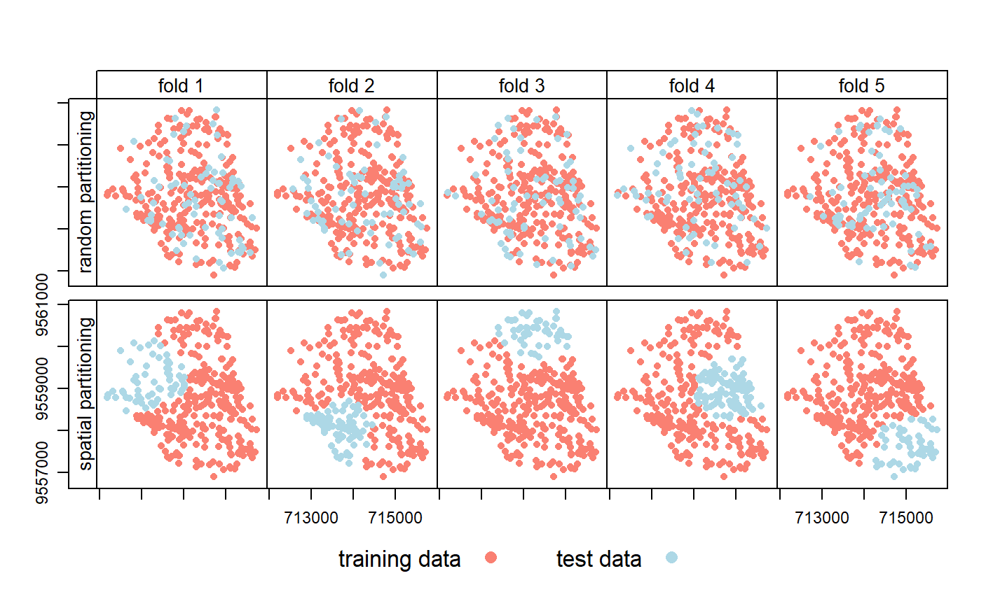
Spatial visualization of selected test and training observations for cross-validation of one repetition. Random (upper row) and spatial partitioning (lower row).

FIGURE 11.3: Spatial visualization of selected test and training observations for cross-validation of one repetition. Random (upper row) and spatial partitioning (lower row).

11.5 Spatial CV with mlr

There are dozens of packages for statistical learning, as described for example in the CRAN machine learning task view. Getting acquainted with each of these packages, including how to undertake cross-validation and hyperparameter tuning, can be a time-consuming process. Comparing model results from different packages can be even more laborious. The mlr package was developed to address these issues. It acts as a ‘meta-package,’ providing a unified interface to popular supervised and unsupervised statistical learning techniques including classification, regression, survival analysis and clustering (Bischl et al. 2016). The standardized mlr interface is based on eight ‘building blocks.’ As illustrated in Figure 11.4, these have a clear order.

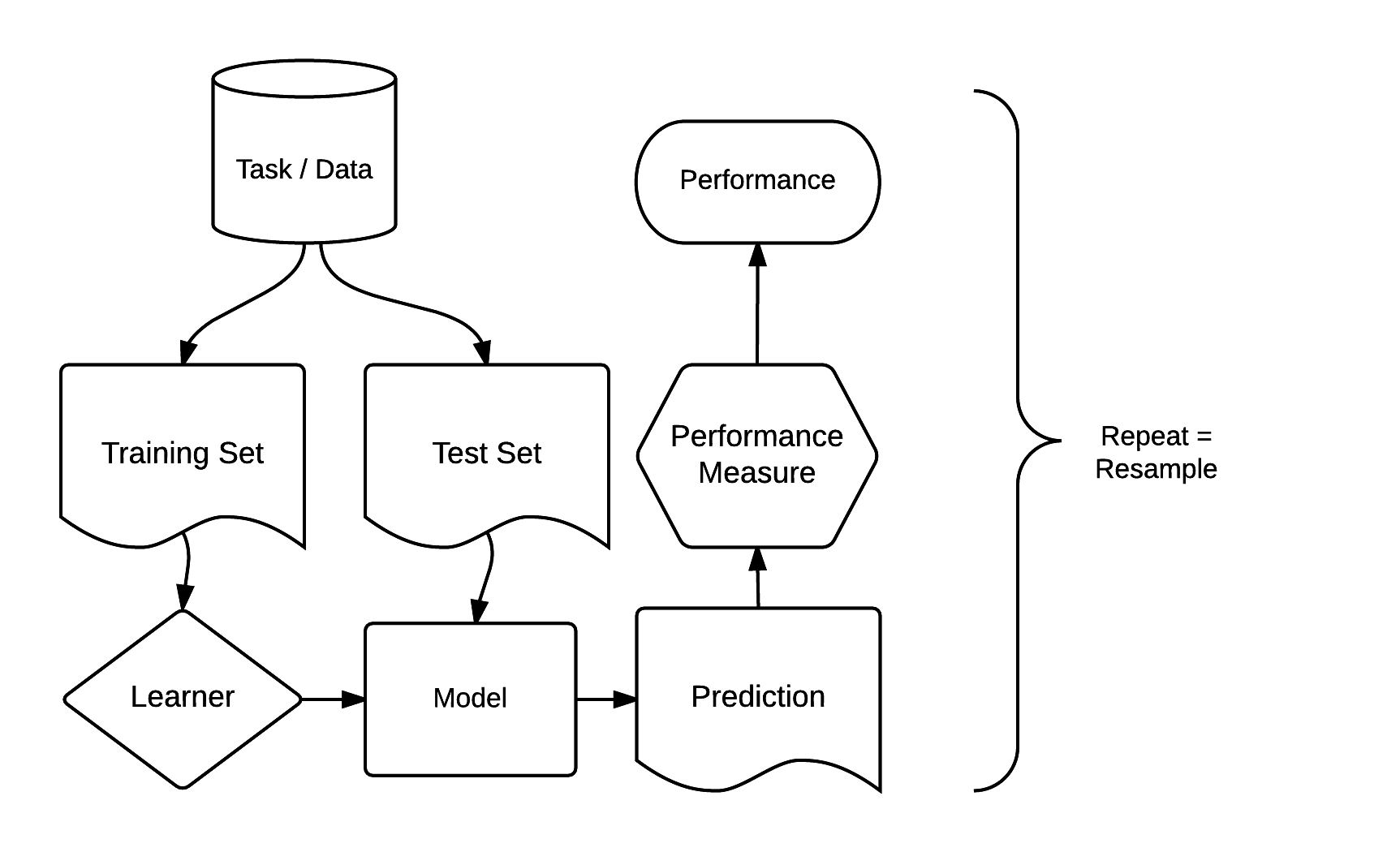
FIGURE 11.4: Basic building blocks of the mlr package. Source: http://bit.ly/2tcb2b7. (Permission to reuse this figure was kindly granted.)

The mlr modeling process consists of three main stages. First, a task specifies the data (including response and predictor variables) and the model type (such as regression or classification). Second, a learner defines the specific learning algorithm that is applied to the created task. Third, the resampling approach assesses the predictive performance of the model, i.e., its ability to generalize to new data (see also Section 11.4).

11.5.1 Generalized linear model

To implement a GLM in mlr, we must create a task containing the landslide data. Since the response is binary (two-category variable), we create a classification task with makeClassifTask() (for regression tasks, use makeRegrTask(), see ?makeRegrTask for other task types). The first essential argument of these make*() functions is data. The target argument expects the name of a response variable and positive determines which of the two factor levels of the response variable indicate the landslide initiation point (in our case this is TRUE). All other variables of the lsl dataset will serve as predictors except for the coordinates (see the result of getTaskFormula(task) for the model formula). For spatial CV, the coordinates parameter is used (see Section 11.4 and Figure 11.3) which expects the coordinates as a xy data frame.

library(mlr)
# coordinates needed for the spatial partitioning
coords = lsl[, c("x", "y")]
# select response and predictors to use in the modeling
data = dplyr::select(lsl, -x, -y)
# create task
task = makeClassifTask(data = data, target = "lslpts",
                       positive = "TRUE", coordinates = coords)

makeLearner() determines the statistical learning method to use. All classification learners start with classif. and all regression learners with regr. (see ?makeLearners for details). listLearners() helps to find out about all available learners and from which package mlr imports them (Table 11.2). For a specific task, we can run:

listLearners(task, warn.missing.packages = FALSE) %>%
  dplyr::select(class, name, short.name, package) %>%
  head()

TABLE 11.2: Sample of available learners for binomial tasks in the mlr package.
Class	Name	Short name	Package
classif.adaboostm1	ada Boosting M1	adaboostm1	RWeka
classif.binomial	Binomial Regression	binomial	stats
classif.featureless	Featureless classifier	featureless	mlr
classif.fnn	Fast k-Nearest Neighbour	fnn	FNN
classif.gausspr	Gaussian Processes	gausspr	kernlab
classif.IBk	k-Nearest Neighbours	ibk	RWeka

This yields all learners able to model two-class problems (landslide yes or no). We opt for the binomial classification method used in Section 11.3 and implemented as classif.binomial in mlr. Additionally, we must specify the link-function, logit in this case, which is also the default of the binomial() function. predict.type determines the type of the prediction with prob resulting in the predicted probability for landslide occurrence between 0 and 1 (this corresponds to type = response in predict.glm).

lrn = makeLearner(cl = "classif.binomial",
                  link = "logit",
                  predict.type = "prob",
                  fix.factors.prediction = TRUE)

To find out from which package the specified learner is taken and how to access the corresponding help pages, we can run:

getLearnerPackages(lrn)
helpLearner(lrn)

The set-up steps for modeling with mlr may seem tedious. But remember, this single interface provides access to the 150+ learners shown by listLearners(); it would be far more tedious to learn the interface for each learner! Further advantages are simple parallelization of resampling techniques and the ability to tune machine learning hyperparameters (see Section 11.5.2). Most importantly, (spatial) resampling in mlr is straightforward, requiring only two more steps: specifying a resampling method and running it. We will use a 100-repeated 5-fold spatial CV: five partitions will be chosen based on the provided coordinates in our task and the partitioning will be repeated 100 times:⁷⁰

perf_level = makeResampleDesc(method = "SpRepCV", folds = 5, reps = 100)

To execute the spatial resampling, we run resample() using the specified learner, task, resampling strategy and of course the performance measure, here the AUROC. This takes some time (around 10 seconds on a modern laptop) because it computes the AUROC for 500 models. Setting a seed ensures the reproducibility of the obtained result and will ensure the same spatial partitioning when re-running the code.

set.seed(012348)
sp_cv = mlr::resample(learner = lrn, task = task,
                      resampling = perf_level, 
                      measures = mlr::auc)

The output of the preceding code chunk is a bias-reduced assessment of the model’s predictive performance, as illustrated in the following code chunk (required input data is saved in the file spatialcv.Rdata in the book’s GitHub repo):

# summary statistics of the 500 models
summary(sp_cv$measures.test$auc)
#>    Min. 1st Qu.  Median    Mean 3rd Qu.    Max. 
#>   0.686   0.757   0.789   0.780   0.795   0.861
# mean AUROC of the 500 models
mean(sp_cv$measures.test$auc)
#> [1] 0.78

To put these results in perspective, let us compare them with AUROC values from a 100-repeated 5-fold non-spatial cross-validation (Figure 11.5; the code for the non-spatial cross-validation is not shown here but will be explored in the exercise section). As expected, the spatially cross-validated result yields lower AUROC values on average than the conventional cross-validation approach, underlining the over-optimistic predictive performance due to spatial autocorrelation of the latter.

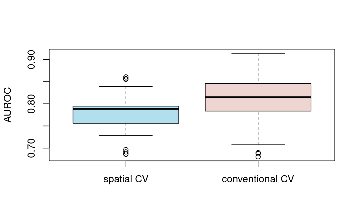
FIGURE 11.5: Boxplot showing the difference in AUROC values between spatial and conventional 100-repeated 5-fold cross-validation.

11.5.2 Spatial tuning of machine-learning hyperparameters

Section 11.4 introduced machine learning as part of statistical learning. To recap, we adhere to the following definition of machine learning by Jason Brownlee:

Machine learning, more specifically the field of predictive modeling, is primarily concerned with minimizing the error of a model or making the most accurate predictions possible, at the expense of explainability. In applied machine learning we will borrow, reuse and steal algorithms from many different fields, including statistics and use them towards these ends.

In Section 11.5.1 a GLM was used to predict landslide susceptibility. This section introduces support vector machines (SVM) for the same purpose. Random forest models might be more popular than SVMs; however, the positive effect of tuning hyperparameters on model performance is much more pronounced in the case of SVMs (Probst, Wright, and Boulesteix 2018). Since (spatial) hyperparameter tuning is the major aim of this section, we will use an SVM. For those wishing to apply a random forest model, we recommend to read this chapter, and then proceed to Chapter 14 in which we will apply the currently covered concepts and techniques to make spatial predictions based on a random forest model.

SVMs search for the best possible ‘hyperplanes’ to separate classes (in a classification case) and estimate ‘kernels’ with specific hyperparameters to allow for non-linear boundaries between classes (James et al. 2013). Hyperparameters should not be confused with coefficients of parametric models, which are sometimes also referred to as parameters.⁷¹ Coefficients can be estimated from the data, while hyperparameters are set before the learning begins. Optimal hyperparameters are usually determined within a defined range with the help of cross-validation methods. This is called hyperparameter tuning.

Some SVM implementations such as that provided by kernlab allow hyperparameters to be tuned automatically, usually based on random sampling (see upper row of Figure 11.3). This works for non-spatial data but is of less use for spatial data where ‘spatial tuning’ should be undertaken.

Before defining spatial tuning, we will set up the mlr building blocks, introduced in Section 11.5.1, for the SVM. The classification task remains the same, hence we can simply reuse the task object created in Section 11.5.1. Learners implementing SVM can be found using listLearners() as follows:

lrns = listLearners(task, warn.missing.packages = FALSE)
filter(lrns, grepl("svm", class)) %>% 
  dplyr::select(class, name, short.name, package)
#>            class                                 name short.name package
#> 6   classif.ksvm              Support Vector Machines       ksvm kernlab
#> 9  classif.lssvm Least Squares Support Vector Machine      lssvm kernlab
#> 17   classif.svm     Support Vector Machines (libsvm)        svm   e1071

Of the options illustrated above, we will use ksvm() from the kernlab package (Karatzoglou et al. 2004). To allow for non-linear relationships, we use the popular radial basis function (or Gaussian) kernel which is also the default of ksvm().

lrn_ksvm = makeLearner("classif.ksvm",
                        predict.type = "prob",
                        kernel = "rbfdot")

The next stage is to specify a resampling strategy. Again we will use a 100-repeated 5-fold spatial CV.

# performance estimation level
perf_level = makeResampleDesc(method = "SpRepCV", folds = 5, reps = 100)

Note that this is the exact same code as used for the GLM in Section 11.5.1; we have simply repeated it here as a reminder.

So far, the process has been identical to that described in Section 11.5.1. The next step is new, however: to tune the hyperparameters. Using the same data for the performance assessment and the tuning would potentially lead to overoptimistic results (Cawley and Talbot 2010). This can be avoided using nested spatial CV.

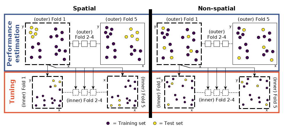
Schematic of hyperparameter tuning and performance estimation levels in CV. (Figure was taken from Schratz et al. (2018). Permission to reuse it was kindly granted.)

FIGURE 11.6: Schematic of hyperparameter tuning and performance estimation levels in CV. (Figure was taken from Schratz et al. (2018). Permission to reuse it was kindly granted.)

This means that we split each fold again into five spatially disjoint subfolds which are used to determine the optimal hyperparameters (tune_level object in the code chunk below; see Figure 11.6 for a visual representation). To find the optimal hyperparameter combination, we fit 50 models (ctrl object in the code chunk below) in each of these subfolds with randomly selected values for the hyperparameters C and Sigma. The random selection of values C and Sigma is additionally restricted to a predefined tuning space (ps object). The range of the tuning space was chosen with values recommended in the literature (Schratz et al. 2018).

# five spatially disjoint partitions
tune_level = makeResampleDesc("SpCV", iters = 5)
# use 50 randomly selected hyperparameters
ctrl = makeTuneControlRandom(maxit = 50)
# define the outer limits of the randomly selected hyperparameters
ps = makeParamSet(
  makeNumericParam("C", lower = -12, upper = 15, trafo = function(x) 2^x),
  makeNumericParam("sigma", lower = -15, upper = 6, trafo = function(x) 2^x)
  )

The next stage is to modify the learner lrn_ksvm in accordance with all the characteristics defining the hyperparameter tuning with makeTuneWrapper().

wrapped_lrn_ksvm = makeTuneWrapper(learner = lrn_ksvm, 
                                   resampling = tune_level,
                                   par.set = ps,
                                   control = ctrl, 
                                   show.info = TRUE,
                                   measures = mlr::auc)

The mlr is now set-up to fit 250 models to determine optimal hyperparameters for one fold. Repeating this for each fold, we end up with 1250 (250 * 5) models for each repetition. Repeated 100 times means fitting a total of 125,000 models to identify optimal hyperparameters (Figure 11.3). These are used in the performance estimation, which requires the fitting of another 500 models (5 folds * 100 repetitions; see Figure 11.3). To make the performance estimation processing chain even clearer, let us write down the commands we have given to the computer:

Performance level (upper left part of Figure 11.6): split the dataset into five spatially disjoint (outer) subfolds.
Tuning level (lower left part of Figure 11.6): use the first fold of the performance level and split it again spatially into five (inner) subfolds for the hyperparameter tuning. Use the 50 randomly selected hyperparameters in each of these inner subfolds, i.e., fit 250 models.
Performance estimation: Use the best hyperparameter combination from the previous step (tuning level) and apply it to the first outer fold in the performance level to estimate the performance (AUROC).
Repeat steps 2 and 3 for the remaining four outer folds.
Repeat steps 2 to 4, 100 times.

The process of hyperparameter tuning and performance estimation is computationally intensive. Model runtime can be reduced with parallelization, which can be done in a number of ways, depending on the operating system.

Before starting the parallelization, we ensure that the processing continues even if one of the models throws an error by setting on.learner.error to warn. This avoids the process stopping just because of one failed model, which is desirable on large model runs. To inspect the failed models once the processing is completed, we dump them:

configureMlr(on.learner.error = "warn", on.error.dump = TRUE)

To start the parallelization, we set the mode to multicore which will use mclapply() in the background on a single machine in the case of a Unix-based operating system.⁷² Equivalenty, parallelStartSocket() enables parallelization under Windows. level defines the level at which to enable parallelization, with mlr.tuneParams determining that the hyperparameter tuning level should be parallelized (see lower left part of Figure 11.6, ?parallelGetRegisteredLevels, and the mlr parallelization tutorial for details). We will use half of the available cores (set with the cpus parameter), a setting that allows possible other users to work on the same high performance computing cluster in case one is used (which was the case when we ran the code). Setting mc.set.seed to TRUE ensures that the randomly chosen hyperparameters during the tuning can be reproduced when running the code again. Unfortunately, mc.set.seed is only available under Unix-based systems.

library(parallelMap)
if (Sys.info()["sysname"] %in% c("Linux", "Darwin")) {
parallelStart(mode = "multicore", 
              # parallelize the hyperparameter tuning level
              level = "mlr.tuneParams", 
              # just use half of the available cores
              cpus = round(parallel::detectCores() / 2),
              mc.set.seed = TRUE)
}

if (Sys.info()["sysname"] == "Windows") {
  parallelStartSocket(level = "mlr.tuneParams",
                      cpus =  round(parallel::detectCores() / 2))
}

Now we are set up for computing the nested spatial CV. Using a seed allows us to recreate the exact same spatial partitions when re-running the code. Specifying the resample() parameters follows the exact same procedure as presented when using a GLM, the only difference being the extract argument. This allows the extraction of the hyperparameter tuning results which is important if we plan follow-up analyses on the tuning. After the processing, it is good practice to explicitly stop the parallelization with parallelStop(). Finally, we save the output object (result) to disk in case we would like to use it another R session. Before running the subsequent code, be aware that it is time-consuming: the 125,500 models took ~1/2hr on a server using 24 cores (see below).

set.seed(12345)
result = mlr::resample(learner = wrapped_lrn_ksvm, 
                       task = task,
                       resampling = perf_level,
                       extract = getTuneResult,
                       measures = mlr::auc)
# stop parallelization
parallelStop()
# save your result, e.g.:
# saveRDS(result, "svm_sp_sp_rbf_50it.rds")

In case you do not want to run the code locally, we have saved a subset of the results in the book’s GitHub repo. They can be loaded as follows:

result = readRDS("extdata/spatial_cv_result.rds")

Note that runtime depends on many aspects: CPU speed, the selected algorithm, the selected number of cores and the dataset.

# Exploring the results
# runtime in minutes
round(result$runtime / 60, 2)
#> [1] 37.4

Even more important than the runtime is the final aggregated AUROC: the model’s ability to discriminate the two classes.

# final aggregated AUROC 
result$aggr
#> auc.test.mean 
#>         0.758
# same as
mean(result$measures.test$auc)
#> [1] 0.758

It appears that the GLM (aggregated AUROC was 0.78) is slightly better than the SVM in this specific case. However, using more than 50 iterations in the random search would probably yield hyperparameters that result in models with a better AUROC (Schratz et al. 2018). On the other hand, increasing the number of random search iterations would also increase the total number of models and thus runtime.

The estimated optimal hyperparameters for each fold at the performance estimation level can also be viewed. The following command shows the best hyperparameter combination of the first fold of the first iteration (recall this results from the first 5 * 50 model runs):

# winning hyperparameters of tuning step, 
# i.e. the best combination out of 50 * 5 models
result$extract[[1]]$x
#> $C
#> [1] 0.458
#> 
#> $sigma
#> [1] 0.023

The estimated hyperparameters have been used for the first fold in the first iteration of the performance estimation level which resulted in the following AUROC value:

result$measures.test[1, ]
#>   iter   auc
#> 1    1 0.799

So far spatial CV has been used to assess the ability of learning algorithms to generalize to unseen data. For spatial predictions, one would tune the hyperparameters on the complete dataset. This will be covered in Chapter 14.

11.6 Conclusions

Resampling methods are an important part of a data scientist’s toolbox (James et al. 2013). This chapter used cross-validation to assess predictive performance of various models. As described in Section 11.4, observations with spatial coordinates may not be statistically independent due to spatial autocorrelation, violating a fundamental assumption of cross-validation. Spatial CV addresses this issue by reducing bias introduced by spatial autocorrelation.

The mlr package facilitates (spatial) resampling techniques in combination with the most popular statistical learning techniques including linear regression, semi-parametric models such as generalized additive models and machine learning techniques such as random forests, SVMs, and boosted regression trees (Bischl et al. 2016; Schratz et al. 2018). Machine learning algorithms often require hyperparameter inputs, the optimal ‘tuning’ of which can require thousands of model runs which require large computational resources, consuming much time, RAM and/or cores. mlr tackles this issue by enabling parallelization.

Machine learning overall, and its use to understand spatial data, is a large field and this chapter has provided the basics, but there is more to learn. We recommend the following resources in this direction:

The mlr tutorials on Machine Learning in R and Handling of spatial Data
An academic paper on hyperparameter tuning (Schratz et al. 2018)
In case of spatio-temporal data, one should account for spatial and temporal autocorrelation when doing CV (Meyer et al. 2018)

11.7 Exercises

Compute the following terrain attributes from the dem datasets loaded with data("landslides", package = "RSAGA") with the help of R-GIS bridges (see Chapter 9):
- Slope
- Plan curvature
- Profile curvature
- Catchment area
Extract the values from the corresponding output rasters to the landslides data frame (data(landslides, package = "RSAGA") by adding new variables called slope, cplan, cprof, elev and log_carea. Keep all landslide initiation points and 175 randomly selected non-landslide points (see Section 11.2 for details).
Use the derived terrain attribute rasters in combination with a GLM to make a spatial prediction map similar to that shown in Figure 11.2. Running data("study_mask", package = "spDataLarge") attaches a mask of the study area.
Compute a 100-repeated 5-fold non-spatial cross-validation and spatial CV based on the GLM learner and compare the AUROC values from both resampling strategies with the help of boxplots (see Figure 11.5). Hint: You need to specify a non-spatial task and a non-spatial resampling strategy.
Model landslide susceptibility using a quadratic discriminant analysis (QDA, James et al. 2013). Assess the predictive performance (AUROC) of the QDA. What is the difference between the spatially cross-validated mean AUROC value of the QDA and the GLM? Hint: Before running the spatial cross-validation for both learners, set a seed to make sure that both use the same spatial partitions which in turn guarantees comparability.
Run the SVM without tuning the hyperparameters. Use the rbfdot kernel with $\sigma$ = 1 and C = 1. Leaving the hyperparameters unspecified in kernlab’s ksvm() would otherwise initialize an automatic non-spatial hyperparameter tuning. For a discussion on the need for (spatial) tuning of hyperparameters, please refer to Schratz et al. (2018).

10 Scripts, algorithms and functions

12 Transportation

Geocomputation with R