9 Bridges to GIS software

Prerequisites

This chapter requires QGIS, SAGA and GRASS to be installed and the following packages to be attached:⁴⁵

library(sf)
library(raster)

#library(RQGIS)
library(RSAGA)
library(rgrass7)

9.1 Introduction

A defining feature of R is the way you interact with it: you type commands and hit Enter (or Ctrl+Enter if writing code in the source editor in RStudio) to execute them interactively. This way of interacting with the computer is called a command-line interface (CLI) (see definition in the note below). CLIs are not unique to R.⁴⁶ In dedicated GIS packages, by contrast, the emphasis tends to be on the graphical user interface (GUI). You can interact with GRASS, QGIS, SAGA and gvSIG from system terminals and embedded CLIs such as the Python Console in QGIS, but ‘pointing and clicking’ is the norm. This means many GIS users miss out on the advantages of the command-line according to Gary Sherman, creator of QGIS (Sherman 2008):

With the advent of ‘modern’ GIS software, most people want to point and click their way through life. That’s good, but there is a tremendous amount of flexibility and power waiting for you with the command line. Many times you can do something on the command line in a fraction of the time you can do it with a GUI.

The ‘CLI vs GUI’ debate can be adversial but it does not have to be; both options can be used interchangeably, depending on the task at hand and the user’s skillset.⁴⁷ The advantages of a good CLI such as that provided by R (and enhanced by IDEs such as RStudio) are numerous. A good CLI:

Facilitates the automation of repetitive tasks;
Enables transparency and reproducibility, the backbone of good scientific practice and data science;
Encourages software development by providing tools to modify existing functions and implement new ones;
Helps develop future-proof programming skills which are in high demand in many disciplines and industries; and
Is user-friendly and fast, allowing an efficient workflow.

On the other hand, GUI-based GIS systems (particularly QGIS) are also advantageous. A good GIS GUI:

Has a ‘shallow’ learning curve meaning geographic data can be explored and visualized without hours of learning a new language;
Provides excellent support for ‘digitizing’ (creating new vector datasets), including trace, snap and topological tools;⁴⁸
Enables georeferencing (matching raster images to existing maps) with ground control points and orthorectification;
Supports stereoscopic mapping (e.g., LiDAR and structure from motion); and
Provides access to spatial database management systems with object-oriented relational data models, topology and fast (spatial) querying.

Another advantage of dedicated GISs is that they provide access to hundreds of ‘geoalgorithms’ (computational recipes to solve geographic problems — see Chapter 10). Many of these are unavailable from the R command line, except via ‘GIS bridges,’ the topic of (and motivation for) this chapter.⁴⁹

A command-line interface is a means of interacting with computer programs in which the user issues commands via successive lines of text (command lines). bash in Linux and PowerShell in Windows are common examples. CLIs can be augmented with IDEs such as RStudio for R, which provides code auto-completion and other features to improve the user experience.

R originated as an interface language. Its predecessor S provided access to statistical algorithms in other languages (particularly FORTRAN), but from an intuitive read-evaluate-print loop (REPL) (Chambers 2016). R continues this tradition with interfaces to numerous languages, notably C++, as described in Chapter 1. R was not designed as a GIS. However, its ability to interface with dedicated GISs gives it astonishing geospatial capabilities. R is well known as a statistical programming language, but many people are unaware of its ability to replicate GIS workflows, with the additional benefits of a (relatively) consistent CLI. Furthermore, R outperforms GISs in some areas of geocomputation, including interactive/animated map making (see Chapter 8) and spatial statistical modeling (see Chapter 11). This chapter focuses on ‘bridges’ to three mature open source GIS products (see Table 9.1): QGIS (via the package RQGIS; Section 9.2), SAGA (via RSAGA; Section 9.3) and GRASS (via rgrass7; Section 9.4). Though not covered here, it is worth being aware of the interface to ArcGIS, a proprietary and very popular GIS software, via RPyGeo.⁵⁰ To complement the R-GIS bridges, the chapter ends with a very brief introduction to interfaces to spatial libraries (Section 9.6.1) and spatial databases (Section 9.6.2).

TABLE 9.1: Comparison between three open-source GIS. Hybrid refers to the support of vector and raster operations.
GIS	First release	No. functions	Support
GRASS	1984	>500	hybrid
QGIS	2002	>1000	hybrid
SAGA	2004	>600	hybrid

9.2 (R)QGIS

QGIS is one of the most popular open-source GIS [Table 9.1; Graser and Olaya (2015)]. Its main advantage lies in the fact that it provides a unified interface to several other open-source GIS. This means that you have access to GDAL, GRASS and SAGA through QGIS (Graser and Olaya 2015). To run all these geoalgorithms (frequently more than 1000 depending on your set-up) outside of the QGIS GUI, QGIS provides a Python API. RQGIS establishes a tunnel to this Python API through the reticulate package. Basically, functions set_env() and open_app() are doing this. Note that it is optional to run set_env() and open_app() since all functions depending on their output will run them automatically if needed. Before running RQGIS, make sure you have installed QGIS and all its (third-party) dependencies such as SAGA and GRASS. To install RQGIS a number of dependencies are required, as described in the install_guide vignette, which covers installation on Windows, Linux and Mac. At the time of writing (autumn 2018) RQGIS only supports the Long Term Release (2.18), but support for QGIS 3 is in the pipeline (see RQGIS3).

#library(RQGIS)
set_env(dev = FALSE)
#> $`root`
#> [1] "C:/OSGeo4W64"
#> ...

Leaving the path-argument of set_env() unspecified will search the computer for a QGIS installation. Hence, it is faster to specify explicitly the path to your QGIS installation. Subsequently, open_app() sets all paths necessary to run QGIS from within R, and finally creates a so-called QGIS custom application (see http://docs.qgis.org/testing/en/docs/pyqgis_developer_cookbook/intro.html#using-pyqgis-in-custom-applications).

open_app()

We are now ready for some QGIS geoprocessing from within R! The example below shows how to unite polygons, a process that unfortunately produces so-called slivers , tiny polygons resulting from overlaps between the inputs that frequently occur in real-world data. We will see how to remove them.

For the union, we use again the incongruent polygons we have already encountered in Section 4.2.5. Both polygon datasets are available in the spData package, and for both we would like to use a geographic CRS (see also Chapter 6).

data("incongruent", "aggregating_zones", package = "spData")
incongr_wgs = st_transform(incongruent, 4326)
aggzone_wgs = st_transform(aggregating_zones, 4326)

To find an algorithm to do this work, find_algorithms() searches all QGIS geoalgorithms using regular expressions. Assuming that the short description of the function contains the word “union”, we can run:

find_algorithms("union", name_only = TRUE)
#> [1] "qgis:union"        "saga:fuzzyunionor" "saga:union"

Short descriptions for each geoalgorithm can also be provided, by setting name_only = FALSE. If one has no clue at all what the name of a geoalgorithm might be, one can leave the search_term-argument empty which will return a list of all available QGIS geoalgorithms. You can also find the algorithms in the QGIS online documentation.

The next step is to find out how qgis:union can be used. open_help() opens the online help of the geoalgorithm in question. get_usage() returns all function parameters and default values.

alg = "qgis:union"
open_help(alg)
get_usage(alg)
#>ALGORITHM: Union
#>  INPUT <ParameterVector>
#>  INPUT2 <ParameterVector>
#>  OUTPUT <OutputVector>

Finally, we can let QGIS do the work. Note that the workhorse function run_qgis() accepts R named arguments, i.e., you can specify the parameter names as returned by get_usage() in run_qgis() as you would do in any other regular R function. Note also that run_qgis() accepts spatial objects residing in R’s global environment as input (here: aggzone_wgs and incongr_wgs). But of course, you could also specify paths to spatial vector files stored on disk. Setting the load_output to TRUE automatically loads the QGIS output as an sf-object into R.

union = run_qgis(alg, INPUT = incongr_wgs, INPUT2 = aggzone_wgs, 
                 OUTPUT = file.path(tempdir(), "union.shp"),
                 load_output = TRUE)
#> $`OUTPUT`
#> [1] "C:/Users/geocompr/AppData/Local/Temp/RtmpcJlnUx/union.shp"

Note that the QGIS union operation merges the two input layers into one layer by using the intersection and the symmetrical difference of the two input layers (which by the way is also the default when doing a union operation in GRASS and SAGA). This is not the same as st_union(incongr_wgs, aggzone_wgs) (see Exercises)! The QGIS output contains empty geometries and multipart polygons. Empty geometries might lead to problems in subsequent geoprocessing tasks which is why they will be deleted. st_dimension() returns NA if a geometry is empty, and can therefore be used as a filter.

# remove empty geometries
union = union[!is.na(st_dimension(union)), ]

Next we convert multipart polygons into single-part polygons (also known as explode geometries or casting). This is necessary for the deletion of sliver polygons later on.

# multipart polygons to single polygons
single = st_cast(union, "POLYGON")

One way to identify slivers is to find polygons with comparatively very small areas, here, e.g., 25000 m² (see blue colored polygons in the left panel of Figure 9.1).

# find polygons which are smaller than 25000 m^2
x = 25000
units(x) = "m^2"
single$area = st_area(single)
sub = dplyr::filter(single, area < x)

The next step is to find a function that makes the slivers disappear. Assuming the function or its short description contains the word “sliver,” we can run:

find_algorithms("sliver", name_only = TRUE)
#> [1] "qgis:eliminatesliverpolygons"

This returns only one geoalgorithm whose parameters can be accessed with the help of get_usage() again.

alg = "qgis:eliminatesliverpolygons"
get_usage(alg)
#>ALGORITHM: Eliminate sliver polygons
#>  INPUT <ParameterVector>
#>  KEEPSELECTION <ParameterBoolean>
#>  ATTRIBUTE <parameters from INPUT>
#>  COMPARISON <ParameterSelection>
#>  COMPARISONVALUE <ParameterString>
#>  MODE <ParameterSelection>
#>  OUTPUT <OutputVector>
#>  ...

Conveniently, the user does not need to specify each single parameter. In case a parameter is left unspecified, run_qgis() will automatically use the corresponding default value as an argument if available. To find out about the default values, run get_args_man().

To remove the slivers, we specify that all polygons with an area less or equal to 25,000 m² should be joined to the neighboring polygon with the largest area (see right panel of Figure 9.1).

clean = run_qgis("qgis:eliminatesliverpolygons",
                 INPUT = single,
                 ATTRIBUTE = "area",
                 COMPARISON = "<=",
                 COMPARISONVALUE = 25000,
                 OUTPUT = file.path(tempdir(), "clean.shp"),
                 load_output = TRUE)
#> $`OUTPUT`
#> [1] "C:/Users/geocompr/AppData/Local/Temp/RtmpcJlnUx/clean.shp"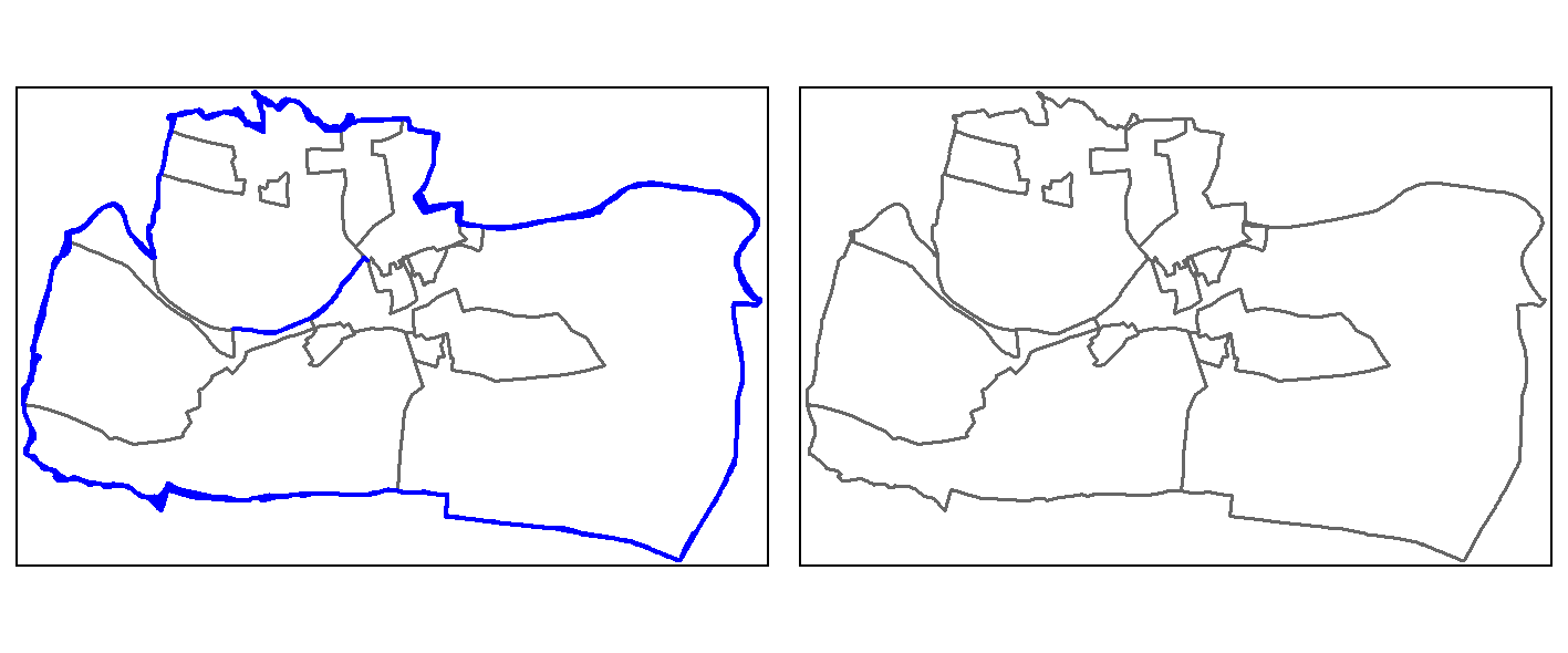

FIGURE 9.1: Sliver polygons colored in blue (left panel). Cleaned polygons (right panel).

In the code chunk above note that

leaving the output parameter(s) unspecified saves the resulting QGIS output to a temporary folder created by QGIS; run_qgis() prints these paths to the console after successfully running the QGIS engine; and
if the output consists of multiple files and you have set load_output to TRUE, run_qgis() will return a list with each element corresponding to one output file.

To learn more about RQGIS, see Muenchow, Schratz, and Brenning (2017).

9.3 (R)SAGA

The System for Automated Geoscientific Analyses (SAGA; Table 9.1) provides the possibility to execute SAGA modules via the command line interface (saga_cmd.exe under Windows and just saga_cmd under Linux) (see the SAGA wiki on modules). In addition, there is a Python interface (SAGA Python API). RSAGA uses the former to run SAGA from within R.

Though SAGA is a hybrid GIS, its main focus has been on raster processing, and here particularly on digital elevation models (soil properties, terrain attributes, climate parameters). Hence, SAGA is especially good at the fast processing of large (high-resolution) raster datasets (Conrad et al. 2015). Therefore, we will introduce RSAGA with a raster use case from Muenchow, Brenning, and Richter (2012). Specifically, we would like to compute the SAGA wetness index from a digital elevation model. First of all, we need to make sure that RSAGA will find SAGA on the computer when called. For this, all RSAGA functions using SAGA in the background make use of rsaga.env(). Usually, rsaga.env() will detect SAGA automatically by searching several likely directories (see its help for more information).

library(RSAGA)
rsaga.env()
#> Search for SAGA command line program and modules... 
#> Done
#> $workspace
#> [1] "."
#> ...

However, it is possible to have ‘hidden’ SAGA in a location rsaga.env() does not search automatically. linkSAGA searches your computer for a valid SAGA installation. If it finds one, it adds the newest version to the PATH environment variable thereby making sure that rsaga.env() runs successfully. It is only necessary to run the next code chunk if rsaga.env() was unsuccessful (see previous code chunk).

library(link2GI)
saga = linkSAGA()
rsaga.env()

Secondly, we need to write the digital elevation model to a SAGA-format. Note that calling data(landslides) attaches two objects to the global environment - dem, a digital elevation model in the form of a list, and landslides, a data.frame containing observations representing the presence or absence of a landslide:

data(landslides)
write.sgrd(data = dem, file = file.path(tempdir(), "dem"), header = dem$header)

The organization of SAGA is modular. Libraries contain so-called modules, i.e., geoalgorithms. To find out which libraries are available, run (output not shown):

rsaga.get.libraries()

We choose the library ta_hydrology (ta is the abbreviation for terrain analysis). Subsequently, we can access the available modules of a specific library (here: ta_hydrology) as follows:

rsaga.get.modules(libs = "ta_hydrology")

rsaga.get.usage() prints the function parameters of a specific geoalgorithm, e.g., the SAGA Wetness Index, to the console.

rsaga.get.usage(lib = "ta_hydrology", module = "SAGA Wetness Index")

Finally, you can run SAGA from within R using RSAGA’s geoprocessing workhorse function rsaga.geoprocessor(). The function expects a parameter-argument list in which you have specified all necessary parameters.

params = list(DEM = file.path(tempdir(), "dem.sgrd"),
              TWI = file.path(tempdir(), "twi.sdat"))
rsaga.geoprocessor(lib = "ta_hydrology", module = "SAGA Wetness Index", 
                   param = params)

To facilitate the access to the SAGA interface, RSAGA frequently provides user-friendly wrapper-functions with meaningful default values (see RSAGA documentation for examples, e.g., ?rsaga.wetness.index). So the function call for calculating the ‘SAGA Wetness Index’ becomes:

rsaga.wetness.index(in.dem = file.path(tempdir(), "dem"), 
                    out.wetness.index = file.path(tempdir(), "twi"))

Of course, we would like to inspect our result visually (Figure 9.2). To load and plot the SAGA output file, we use the raster package.

library(raster)
twi = raster::raster(file.path(tempdir(), "twi.sdat"))
# shown is a version using tmap
plot(twi, col = RColorBrewer::brewer.pal(n = 9, name = "Blues"))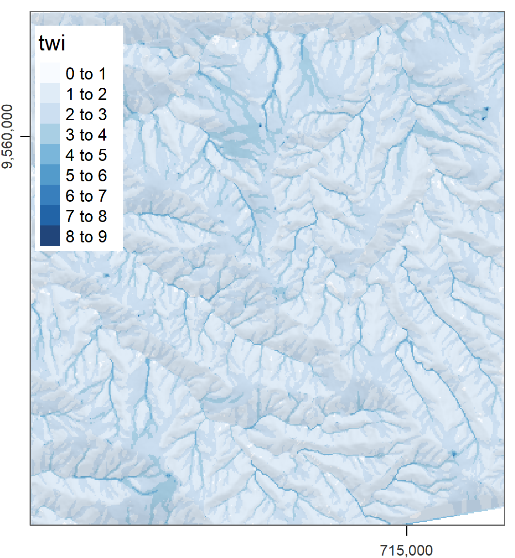

FIGURE 9.2: SAGA wetness index of Mount Mongón, Peru.

You can find an extended version of this example in vignette("RSAGA-landslides") which includes the use of statistical geocomputing to derive terrain attributes as predictors for a non-linear Generalized Additive Model (GAM) to predict spatially landslide susceptibility (Muenchow, Brenning, and Richter 2012). The term statistical geocomputation emphasizes the strength of combining R’s data science power with the geoprocessing power of a GIS which is at the very heart of building a bridge from R to GIS.

9.4 GRASS through rgrass7

The U.S. Army - Construction Engineering Research Laboratory (USA-CERL) created the core of the Geographical Resources Analysis Support System (GRASS) [Table 9.1; Neteler and Mitasova (2008)] from 1982 to 1995. Academia continued this work since 1997. Similar to SAGA, GRASS focused on raster processing in the beginning while only later, since GRASS 6.0, adding advanced vector functionality (R. Bivand, Pebesma, and Gómez-Rubio 2013).

We will introduce rgrass7 with one of the most interesting problems in GIScience - the traveling salesman problem. Suppose a traveling salesman would like to visit 24 customers. Additionally, he would like to start and finish his journey at home which makes a total of 25 locations while covering the shortest distance possible. There is a single best solution to this problem; however, to find it is even for modern computers (mostly) impossible (P. Longley 2015). In our case, the number of possible solutions correspond to (25 - 1)! / 2, i.e., the factorial of 24 divided by 2 (since we do not differentiate between forward or backward direction). Even if one iteration can be done in a nanosecond, this still corresponds to 9837145 years. Luckily, there are clever, almost optimal solutions which run in a tiny fraction of this inconceivable amount of time. GRASS GIS provides one of these solutions (for more details, see v.net.salesman). In our use case, we would like to find the shortest path between the first 25 bicycle stations (instead of customers) on London’s streets (and we simply assume that the first bike station corresponds to the home of our traveling salesman).

data("cycle_hire", package = "spData")
points = cycle_hire[1:25, ]

Aside from the cycle hire points data, we will need the OpenStreetMap data of London. We download it with the help of the osmdata package (see also Section 7.2). We constrain the download of the street network (in OSM language called “highway”) to the bounding box of the cycle hire data, and attach the corresponding data as an sf-object. osmdata_sf() returns a list with several spatial objects (points, lines, polygons, etc.). Here, we will only keep the line objects. OpenStreetMap objects come with a lot of columns, streets features almost 500. In fact, we are only interested in the geometry column. Nevertheless, we are keeping one attribute column; otherwise, we will run into trouble when trying to provide writeVECT() only with a geometry object (see further below and ?writeVECT for more details). Remember that the geometry column is sticky, hence, even though we are just selecting one attribute, the geometry column will be also returned (see Section 2.2.1).

library(osmdata)
b_box = st_bbox(points)
london_streets = opq(b_box) %>%
  add_osm_feature(key = "highway") %>%
  osmdata_sf() %>%
  `[[`("osm_lines")
london_streets = dplyr::select(london_streets, osm_id)

As a convenience to the reader, one can attach london_streets to the global environment using data("london_streets", package = "spDataLarge").

Now that we have the data, we can go on and initiate a GRASS session, i.e., we have to create a GRASS spatial database. The GRASS geodatabase system is based on SQLite. Consequently, different users can easily work on the same project, possibly with different read/write permissions. However, one has to set up this spatial database (also from within R), and users used to a GIS GUI popping up by one click might find this process a bit intimidating in the beginning. First of all, the GRASS database requires its own directory, and contains a location (see the GRASS GIS Database help pages at grass.osgeo.org for further information). The location in turn simply contains the geodata for one project. Within one location, several mapsets can exist and typically refer to different users. PERMANENT is a mandatory mapset and is created automatically. It stores the projection, the spatial extent and the default resolution for raster data. In order to share geographic data with all users of a project, the database owner can add spatial data to the PERMANENT mapset. Please refer to Neteler and Mitasova (2008) and the GRASS GIS quick start for more information on the GRASS spatial database system.

You have to set up a location and a mapset if you want to use GRASS from within R. First of all, we need to find out if and where GRASS 7 is installed on the computer.

library(link2GI)
link = findGRASS()

link is a data.frame which contains in its rows the GRASS 7 installations on your computer. Here, we will use a GRASS 7 installation. If you have not installed GRASS 7 on your computer, we recommend that you do so now. Assuming that we have found a working installation on your computer, we use the corresponding path in initGRASS. Additionally, we specify where to store the spatial database (gisDbase), name the location london, and use the PERMANENT mapset.

library(rgrass7)
# find a GRASS 7 installation, and use the first one
ind = grep("7", link$version)[1]
# next line of code only necessary if we want to use GRASS as installed by 
# OSGeo4W. Among others, this adds some paths to PATH, which are also needed
# for running GRASS.
link2GI::paramGRASSw(link[ind, ])
grass_path = 
  ifelse(test = !is.null(link$installation_type) && 
           link$installation_type[ind] == "osgeo4W",
         yes = file.path(link$instDir[ind], "apps/grass", link$version[ind]),
         no = link$instDir)
initGRASS(gisBase = grass_path,
          # home parameter necessary under UNIX-based systems
          home = tempdir(),
          gisDbase = tempdir(), location = "london", 
          mapset = "PERMANENT", override = TRUE)

Subsequently, we define the projection, the extent and the resolution.

execGRASS("g.proj", flags = c("c", "quiet"), 
          proj4 = st_crs(london_streets)$proj4string)
b_box = st_bbox(london_streets) 
execGRASS("g.region", flags = c("quiet"), 
          n = as.character(b_box["ymax"]), s = as.character(b_box["ymin"]), 
          e = as.character(b_box["xmax"]), w = as.character(b_box["xmin"]), 
          res = "1")

Once you are familiar with how to set up the GRASS environment, it becomes tedious to do so over and over again. Luckily, linkGRASS7() of the link2GI packages lets you do it with one line of code. The only thing you need to provide is a spatial object which determines the projection and the extent of the spatial database.. First, linkGRASS7() finds all GRASS installations on your computer. Since we have set ver_select to TRUE, we can interactively choose one of the found GRASS-installations. If there is just one installation, the linkGRASS7() automatically chooses this one. Second, linkGRASS7() establishes a connection to GRASS 7.

link2GI::linkGRASS7(london_streets, ver_select = TRUE)

Before we can use GRASS geoalgorithms, we need to add data to GRASS’s spatial database. Luckily, the convenience function writeVECT() does this for us. (Use writeRAST() in the case of raster data.) In our case we add the street and cycle hire point data while using only the first attribute column, and name them also london_streets and points.

To use sf-objects with rgrass7, we have to run use_sf() first (note: the code below assumes you are running rgrass7 0.2.1 or above).

use_sf()
writeVECT(SDF = london_streets, vname = "london_streets")
writeVECT(SDF = points[, 1], vname = "points")

To perform our network analysis, we need a topological clean street network. GRASS’s v.clean takes care of the removal of duplicates, small angles and dangles, among others. Here, we break lines at each intersection to ensure that the subsequent routing algorithm can actually turn right or left at an intersection, and save the output in a GRASS object named streets_clean. It is likely that a few of our cycling station points will not lie exactly on a street segment. However, to find the shortest route between them, we need to connect them to the nearest streets segment. v.net’s connect-operator does exactly this. We save its output in streets_points_con.

# clean street network
execGRASS(cmd = "v.clean", input = "london_streets", output = "streets_clean",
          tool = "break", flags = "overwrite")
# connect points with street network
execGRASS(cmd = "v.net", input = "streets_clean", output = "streets_points_con", 
          points = "points", operation = "connect", threshold = 0.001,
          flags = c("overwrite", "c"))

The resulting clean dataset serves as input for the v.net.salesman-algorithm, which finally finds the shortest route between all cycle hire stations. center_cats requires a numeric range as input. This range represents the points for which a shortest route should be calculated. Since we would like to calculate the route for all cycle stations, we set it to 1-25. To access the GRASS help page of the traveling salesman algorithm, run execGRASS("g.manual", entry = "v.net.salesman").

execGRASS(cmd = "v.net.salesman", input = "streets_points_con",
          output = "shortest_route", center_cats = paste0("1-", nrow(points)),
          flags = c("overwrite"))

To visualize our result, we import the output layer into R, convert it into an sf-object keeping only the geometry, and visualize it with the help of the mapview package (Figure 9.3 and Section 8.4).

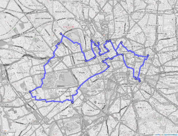
FIGURE 9.3: Shortest route (blue line) between 24 cycle hire stations (blue dots) on the OSM street network of London.

route = readVECT("shortest_route") %>%
  st_as_sf() %>%
  st_geometry()
mapview::mapview(route, map.types = "OpenStreetMap.BlackAndWhite", lwd = 7) +
  points

There are a few important considerations to note in the process:

We could have used GRASS’s spatial database (based on SQLite) which allows faster processing. That means we have only exported geographic data at the beginning. Then we created new objects but only imported the final result back into R. To find out which datasets are currently available, run execGRASS("g.list", type = "vector,raster", flags = "p").
We could have also accessed an already existing GRASS spatial database from within R. Prior to importing data into R, you might want to perform some (spatial) subsetting. Use v.select and v.extract for vector data. db.select lets you select subsets of the attribute table of a vector layer without returning the corresponding geometry.
You can also start R from within a running GRASS session (for more information please refer to R. Bivand, Pebesma, and Gómez-Rubio 2013 and this wiki).
Refer to the excellent GRASS online help or execGRASS("g.manual", flags = "i") for more information on each available GRASS geoalgorithm.
If you would like to use GRASS 6 from within R, use the R package spgrass6.

9.5 When to use what?

To recommend a single R-GIS interface is hard since the usage depends on personal preferences, the tasks at hand and your familiarity with different GIS software packages which in turn probably depends on your field of study. As mentioned previously, SAGA is especially good at the fast processing of large (high-resolution) raster datasets, and frequently used by hydrologists, climatologists and soil scientists (Conrad et al. 2015). GRASS GIS, on the other hand, is the only GIS presented here supporting a topologically based spatial database which is especially useful for network analyses but also simulation studies (see below). QGIS is much more user-friendly compared to GRASS- and SAGA-GIS, especially for first-time GIS users, and probably the most popular open-source GIS. Therefore, RQGIS is an appropriate choice for most use cases. Its main advantages are

a unified access to several GIS, and therefore the provision of >1000 geoalgorithms (Table 9.1) including duplicated functionality, e.g., you can perform overlay-operations using QGIS-, SAGA- or GRASS-geoalgorithms;
automatic data format conversions (SAGA uses .sdat grid files and GRASS uses its own database format but QGIS will handle the corresponding conversions);
its automatic passing of geographic R objects to QGIS geoalgorithms and back into R; and
convenience functions to support the access of the online help, named arguments and automatic default value retrieval (rgrass7 inspired the latter two features).

By all means, there are use cases when you certainly should use one of the other R-GIS bridges. Though QGIS is the only GIS providing a unified interface to several GIS software packages, it only provides access to a subset of the corresponding third-party geoalgorithms (for more information please refer to Muenchow, Schratz, and Brenning (2017)). Therefore, to use the complete set of SAGA and GRASS functions, stick with RSAGA and rgrass7. When doing so, take advantage of RSAGA’s numerous user-friendly functions. Note also, that RSAGA offers native R functions for geocomputation such as multi.local.function(), pick.from.points() and many more. RSAGA supports much more SAGA versions than (R)QGIS. Finally, if you need topological correct data and/or spatial database management functionality such as multi-user access, we recommend the usage of GRASS. In addition, if you would like to run simulations with the help of a geodatabase (Krug, Roura-Pascual, and Richardson 2010), use rgrass7 directly since RQGIS always starts a new GRASS session for each call.

Please note that there are a number of further GIS software packages that have a scripting interface but for which there is no dedicated R package that accesses these: gvSig, OpenJump, Orfeo Toolbox and TauDEM.

9.6 Other bridges

The focus of this chapter is on R interfaces to Desktop GIS software. We emphasize these bridges because dedicated GIS software is well-known and a common ‘way in’ to understanding geographic data. They also provide access to many geoalgorithms.

Other ‘bridges’ include interfaces to spatial libraries (Section 9.6.1 shows how to access the GDAL CLI from R), spatial databases (see Section 9.6.2) and web mapping services (see Chapter 8). This section provides only a snippet of what is possible. Thanks to R’s flexibility, with its ability to call other programs from the system and integration with other languages (notably via Rcpp and reticulate), many other bridges are possible. The aim is not to be comprehensive, but to demonstrate other ways of accessing the ‘flexibility and power’ in the quote by Sherman (2008) at the beginning of the chapter.

9.6.1 Bridges to GDAL

As discussed in Chapter 7, GDAL is a low-level library that supports many geographic data formats. GDAL is so effective that most GIS programs use GDAL in the background for importing and exporting geographic data, rather than re-inventing the wheel and using bespoke read-write code. But GDAL offers more than data I/O. It has geoprocessing tools for vector and raster data, functionality to create tiles for serving raster data online, and rapid rasterization of vector data, all of which can be accessed via the system of R command line.

The code chunk below demonstrates this functionality: linkGDAL() searches the computer for a working GDAL installation and adds the location of the executable files to the PATH variable, allowing GDAL to be called. In the example below ogrinfo provides metadata on a vector dataset:

link2GI::linkGDAL()
cmd = paste("ogrinfo -ro -so -al", system.file("shape/nc.shp", package = "sf"))
system(cmd)
#> INFO: Open of `C:/Users/geocompr/Documents/R/win-library/3.5/sf/shape/nc.shp'
#>     using driver `ESRI Shapefile' successful.
#> 
#> Layer name: nc
#> Metadata:
#>  DBF_DATE_LAST_UPDATE=2016-10-26
#> Geometry: Polygon
#> Feature Count: 100
#> Extent: (-84.323853, 33.881992) - (-75.456978, 36.589649)
#> Layer SRS WKT:
#> ...

This example — which returns the same result as rgdal::ogrInfo() — may be simple, but it shows how to use GDAL via the system command-line, independently of other packages. The ‘link’ to GDAL provided by link2gi could be used as a foundation for doing more advanced GDAL work from the R or system CLI.⁵¹ TauDEM (http://hydrology.usu.edu/taudem/taudem5/index.html) and the Orfeo Toolbox (https://www.orfeo-toolbox.org/) are other spatial data processing libraries/programs offering a command line interface. At the time of writing, it appears that there is only a developer version of an R/TauDEM interface on R-Forge (https://r-forge.r-project.org/R/?group_id=956). In any case, the above example shows how to access these libraries from the system command line via R. This in turn could be the starting point for creating a proper interface to these libraries in the form of new R packages.

Before diving into a project to create a new bridge, however, it is important to be aware of the power of existing R packages and that system() calls may not be platform-independent (they may fail on some computers). Furthermore, sf brings most of the power provided by GDAL, GEOS and PROJ to R via the R/C++ interface provided by Rcpp, which avoids system() calls.

9.6.2 Bridges to spatial databases

Spatial database management systems (spatial DBMS) store spatial and non-spatial data in a structured way. They can organize large collections of data into related tables (entities) via unique identifiers (primary and foreign keys) and implicitly via space (think for instance of a spatial join). This is useful because geographic datasets tend to become big and messy quite quickly. Databases enable storing and querying large datasets efficiently based on spatial and non-spatial fields, and provide multi-user access and topology support.

The most important open source spatial database is PostGIS (Obe and Hsu 2015).⁵² R bridges to spatial DBMSs such as PostGIS are important, allowing access to huge data stores without loading several gigabytes of geographic data into RAM, and likely crashing the R session. The remainder of this section shows how PostGIS can be called from R, based on “Hello real word” from PostGIS in Action, Second Edition (Obe and Hsu 2015).⁵³

The subsequent code requires a working internet connection, since we are accessing a PostgreSQL/PostGIS database which is living in the QGIS Cloud (https://qgiscloud.com/).⁵⁴

library(RPostgreSQL)
conn = dbConnect(drv = PostgreSQL(), dbname = "rtafdf_zljbqm",
                 host = "db.qgiscloud.com",
                 port = "5432", user = "rtafdf_zljbqm", 
                 password = "d3290ead")

Often the first question is, ‘which tables can be found in the database?’ This can be asked as follows (the answer is 5 tables):

dbListTables(conn)
#> [1] "spatial_ref_sys" "topology"        "layer"           "restaurants"    
#> [5] "highways"

We are only interested in the restaurants and the highways tables. The former represents the locations of fast-food restaurants in the US, and the latter are principal US highways. To find out about attributes available in a table, we can run:

dbListFields(conn, "highways")
#> [1] "qc_id"        "wkb_geometry" "gid"          "feature"     
#> [5] "name"         "state"

The first query will select US Route 1 in Maryland (MD). Note that st_read() allows us to read geographic data from a database if it is provided with an open connection to a database and a query. Additionally, st_read() needs to know which column represents the geometry (here: wkb_geometry).

query = paste(
  "SELECT *",
  "FROM highways",
  "WHERE name = 'US Route 1' AND state = 'MD';")
us_route = st_read(conn, query = query, geom = "wkb_geometry")

This results in an sf-object named us_route of type sfc_MULTILINESTRING. The next step is to add a 20-mile buffer (corresponds to 1609 meters times 20) around the selected highway (Figure 9.4).

query = paste(
  "SELECT ST_Union(ST_Buffer(wkb_geometry, 1609 * 20))::geometry",
  "FROM highways",
  "WHERE name = 'US Route 1' AND state = 'MD';")
buf = st_read(conn, query = query)

Note that this was a spatial query using functions (ST_Union(), ST_Buffer()) you should be already familiar with since you find them also in the sf-package, though here they are written in lowercase characters (st_union(), st_buffer()). In fact, function names of the sf package largely follow the PostGIS naming conventions.⁵⁵ The last query will find all Hardee restaurants (HDE) within the buffer zone (Figure 9.4).

query = paste(
  "SELECT r.wkb_geometry",
  "FROM restaurants r",
  "WHERE EXISTS (",
  "SELECT gid",
  "FROM highways",
  "WHERE",
  "ST_DWithin(r.wkb_geometry, wkb_geometry, 1609 * 20) AND",
  "name = 'US Route 1' AND",
  "state = 'MD' AND",
  "r.franchise = 'HDE');"
)
hardees = st_read(conn, query = query)

Please refer to Obe and Hsu (2015) for a detailed explanation of the spatial SQL query. Finally, it is good practice to close the database connection as follows:⁵⁶

RPostgreSQL::postgresqlCloseConnection(conn)

#> old-style crs object detected; please recreate object with a recent sf::st_crs()
#> old-style crs object detected; please recreate object with a recent sf::st_crs()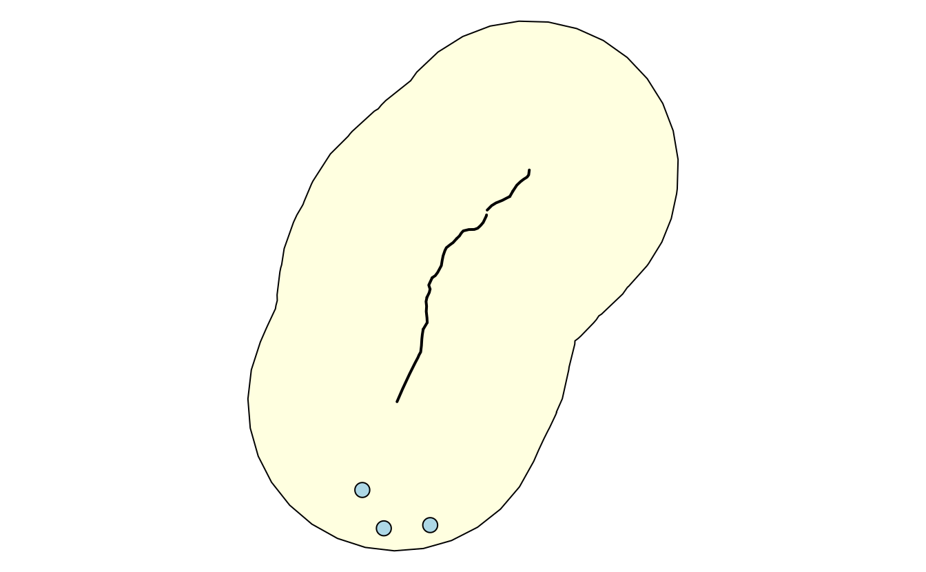

Visualization of the output of previous PostGIS commands showing the highway (black line), a buffer (light yellow) and three restaurants (light blue points) within the buffer.

FIGURE 9.4: Visualization of the output of previous PostGIS commands showing the highway (black line), a buffer (light yellow) and three restaurants (light blue points) within the buffer.

Unlike PostGIS, sf only supports spatial vector data. To query and manipulate raster data stored in a PostGIS database, use the rpostgis package (Bucklin and Basille 2018) and/or use command-line tools such as rastertopgsql which comes as part of the PostGIS installation.

This subsection is only a brief introduction to PostgreSQL/PostGIS. Nevertheless, we would like to encourage the practice of storing geographic and non-geographic data in a spatial DBMS while only attaching those subsets to R’s global environment which are needed for further (geo-)statistical analysis. Please refer to Obe and Hsu (2015) for a more detailed description of the SQL queries presented and a more comprehensive introduction to PostgreSQL/PostGIS in general. PostgreSQL/PostGIS is a formidable choice as an open-source spatial database. But the same is true for the lightweight SQLite/SpatiaLite database engine and GRASS which uses SQLite in the background (see Section 9.4).

As a final note, if your data is getting too big for PostgreSQL/PostGIS and you require massive spatial data management and query performance, then the next logical step is to use large-scale geographic querying on distributed computing systems, as for example, provided by GeoMesa (http://www.geomesa.org/) or GeoSpark [http://geospark.datasyslab.org/; Huang et al. (2017)].

9.7 Exercises

Create two overlapping polygons (poly_1 and poly_2) with the help of the sf-package (see Chapter 2).
Union poly_1 and poly_2 using st_union() and qgis:union. What is the difference between the two union operations? How can we use the sf package to obtain the same result as QGIS?
Calculate the intersection of poly_1 and poly_2 using:
- RQGIS, RSAGA and rgrass7
- sf
Attach data(dem, package = "spDataLarge") and data(random_points, package = "spDataLarge"). Select randomly a point from random_points and find all dem pixels that can be seen from this point (hint: viewshed). Visualize your result. For example, plot a hillshade, and on top of it the digital elevation model, your viewshed output and the point. Additionally, give mapview a try.
Compute catchment area and catchment slope of data("dem", package = "spDataLarge") using RSAGA (see Section 9.3).
Use gdalinfo via a system call for a raster file stored on disk of your choice (see Section 9.6.1).
Query all Californian highways from the PostgreSQL/PostGIS database living in the QGIS Cloud introduced in this chapter (see Section 9.6.2).

8 Making maps with R

10 Scripts, algorithms and functions

Geocomputation with R