14 Ecology

Prerequisites

This chapter assumes you have a strong grasp of geographic data analysis and processing, covered in Chapters 2 to 5. In it you will also make use of R’s interfaces to dedicated GIS software, and spatial cross-validation, topics covered in Chapters 9 and 11, respectively.

The chapter uses the following packages:

library(sf)
library(raster)
# library(RQGIS)
library(mlr)
library(dplyr)
library(vegan)

14.1 Introduction

In this chapter we will model the floristic gradient of fog oases to reveal distinctive vegetation belts that are clearly controlled by water availability. To do so, we will bring together concepts presented in previous chapters and even extend them (Chapters 2 to 5 and Chapters 9 and 11).

Fog oases are one of the most fascinating vegetation formations we have ever encountered. These formations, locally termed lomas, develop on mountains along the coastal deserts of Peru and Chile.⁸² The deserts’ extreme conditions and remoteness provide the habitat for a unique ecosystem, including species endemic to the fog oases. Despite the arid conditions and low levels of precipitation of around 30-50 mm per year on average, fog deposition increases the amount of water available to plants during austal winter. This results in green southern-facing mountain slopes along the coastal strip of Peru (Figure 14.1). This fog, which develops below the temperature inversion caused by the cold Humboldt current in austral winter, provides the name for this habitat. Every few years, the El Niño phenomenon brings torrential rainfall to this sun-baked environment (Dillon, Nakazawa, and Leiva 2003). This causes the desert to bloom, and provides tree seedlings a chance to develop roots long enough to survive the following arid conditions.

Unfortunately, fog oases are heavily endangered. This is mostly due to human activity (agriculture and climate change). To effectively protect the last remnants of this unique vegetation ecosystem, evidence is needed on the composition and spatial distribution of the native flora (Muenchow, Bräuning, et al. 2013; Muenchow, Hauenstein, et al. 2013). Lomas mountains also have economic value as a tourist destination, and can contribute to the well-being of local people via recreation. For example, most Peruvians live in the coastal desert, and lomas mountains are frequently the closest “green” destination.

In this chapter we will demonstrate ecological applications of some of the techniques learned in the previous chapters. This case study will involve analyzing the composition and the spatial distribution of the vascular plants on the southern slope of Mt. Mongón, a lomas mountain near Casma on the central northern coast of Peru (Figure 14.1).

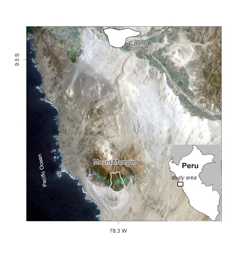
FIGURE 14.1: The Mt. Mongón study area, from Muenchow, Schratz, and Brenning (2017).

During a field study to Mt. Mongón, we recorded all vascular plants living in 100 randomly sampled 4x4 m² plots in the austral winter of 2011 (Muenchow, Bräuning, et al. 2013). The sampling coincided with a strong La Niña event that year (see ENSO monitoring of the NOASS Climate Prediction Center). This led to even higher levels of aridity than usual in the coastal desert. On the other hand, it also increased fog activity on the southern slopes of Peruvian lomas mountains.

Ordinations are dimension-reducing techniques which allow the extraction of the main gradients from a (noisy) dataset, in our case the floristic gradient developing along the southern mountain slope (see next section). In this chapter we will model the first ordination axis, i.e., the floristic gradient, as a function of environmental predictors such as altitude, slope, catchment area and NDVI. For this, we will make use of a random forest model - a very popular machine learning algorithm (Breiman 2001). The model will allow us to make spatial predictions of the floristic composition anywhere in the study area. To guarantee an optimal prediction, it is advisable to tune beforehand the hyperparameters with the help of spatial cross-validation (see Section 11.5.2).

14.2 Data and data preparation

All the data needed for the subsequent analyses is available via the spDataLarge package.

data("study_area", "random_points", "comm", "dem", "ndvi", package = "spDataLarge")

study_area is an sf polygon representing the outlines of the study area. random_points is an sf object, and contains the 100 randomly chosen sites. comm is a community matrix of the wide data format (Wickham 2014) where the rows represent the visited sites in the field and the columns the observed species.⁸³

# sites 35 to 40 and corresponding occurrences of the first five species in the
# community matrix
comm[35:40, 1:5]
#>    Alon_meri Alst_line Alte_hali Alte_porr Anth_eccr
#> 35         0         0         0       0.0     1.000
#> 36         0         0         1       0.0     0.500
#> 37         0         0         0       0.0     0.125
#> 38         0         0         0       0.0     3.000
#> 39         0         0         0       0.0     2.000
#> 40         0         0         0       0.2     0.125

The values represent species cover per site, and were recorded as the area covered by a species in proportion to the site area in percentage points (%; please note that one site can have >100% due to overlapping cover between individual plants). The rownames of comm correspond to the id column of random_points. dem is the digital elevation model (DEM) for the study area, and ndvi is the Normalized Difference Vegetation Index (NDVI) computed from the red and near-infrared channels of a Landsat scene (see Section 4.3.3 and ?ndvi). Visualizing the data helps to get more familiar with it, as shown in Figure 14.2 where the dem is overplotted by the random_points and the study_area.

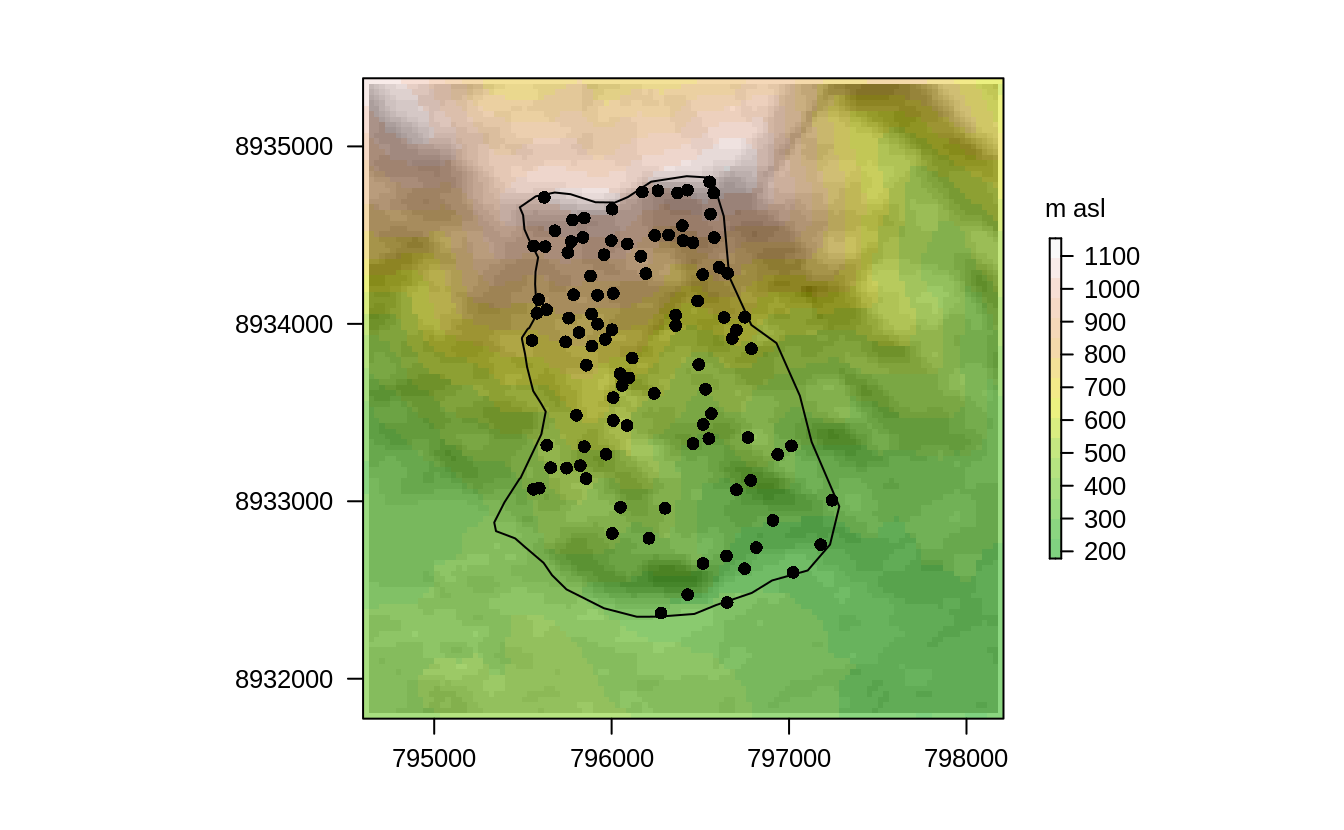
FIGURE 14.2: Study mask (polygon), location of the sampling sites (black points) and DEM in the background.

The next step is to compute variables which we will not only need for the modeling and predictive mapping (see Section 14.4.2) but also for aligning the Non-metric multidimensional scaling (NMDS) axes with the main gradient in the study area, altitude and humidity, respectively (see Section 14.3).

Specifically, we will compute catchment slope and catchment area from a digital elevation model using R-GIS bridges (see Chapter 9). Curvatures might also represent valuable predictors, in the Exercise section you can find out how they would change the modeling result.

To compute catchment area and catchment slope, we will make use of the saga:sagawetnessindex function.⁸⁴ get_usage() returns all function parameters and default values of a specific geoalgorithm. Here, we present only a selection of the complete output.

get_usage("saga:sagawetnessindex")
#>ALGORITHM: Saga wetness index
#>  DEM <ParameterRaster>
#>  ...
#>  SLOPE_TYPE <ParameterSelection>
#>  ...
#>  AREA <OutputRaster>
#>  SLOPE <OutputRaster>
#>  AREA_MOD <OutputRaster>
#>  TWI <OutputRaster>
#> ...
#>SLOPE_TYPE(Type of Slope)
#>  0 - [0] local slope
#>  1 - [1] catchment slope
#> ...

Subsequently, we can specify the needed parameters using R named arguments (see Section 9.2). Remember that we can use a RasterLayer living in R’s global environment to specify the input raster DEM (see Section 9.2). Specifying 1 as the SLOPE_TYPE makes sure that the algorithm will return the catchment slope. The resulting output rasters should be saved to temporary files with an .sdat extension which is a SAGA raster format. Setting load_output to TRUE ensures that the resulting rasters will be imported into R.

# environmental predictors: catchment slope and catchment area
ep = run_qgis(alg = "saga:sagawetnessindex",
              DEM = dem,
              SLOPE_TYPE = 1, 
              SLOPE = tempfile(fileext = ".sdat"),
              AREA = tempfile(fileext = ".sdat"),
              load_output = TRUE,
              show_output_paths = FALSE)

This returns a list named ep consisting of two elements: AREA and SLOPE. Let us add two more raster objects to the list, namely dem and ndvi, and convert it into a raster stack (see Section 2.3.4).

ep = stack(c(dem, ndvi, ep))
names(ep) = c("dem", "ndvi", "carea", "cslope")

Additionally, the catchment area values are highly skewed to the right (hist(ep$carea)). A log10-transformation makes the distribution more normal.

ep$carea = log10(ep$carea)

As a convenience to the reader, we have added ep to spDataLarge:

data("ep", package = "spDataLarge")

Finally, we can extract the terrain attributes to our field observations (see also Section 5.4.2).

random_points[, names(ep)] = raster::extract(ep, random_points)

14.3 Reducing dimensionality

Ordinations are a popular tool in vegetation science to extract the main information, frequently corresponding to ecological gradients, from large species-plot matrices mostly filled with 0s. However, they are also used in remote sensing, the soil sciences, geomarketing and many other fields. If you are unfamiliar with ordination techniques or in need of a refresher, have a look at Michael W. Palmer’s web page for a short introduction to popular ordination techniques in ecology and at Borcard, Gillet, and Legendre (2011) for a deeper look on how to apply these techniques in R. vegan’s package documentation is also a very helpful resource (vignette(package = "vegan")).

Principal component analysis (PCA) is probably the most famous ordination technique. It is a great tool to reduce dimensionality if one can expect linear relationships between variables, and if the joint absence of a variable (for example calcium) in two plots (observations) can be considered a similarity. This is barely the case with vegetation data.

For one, relationships are usually non-linear along environmental gradients. That means the presence of a plant usually follows a unimodal relationship along a gradient (e.g., humidity, temperature or salinity) with a peak at the most favorable conditions and declining ends towards the unfavorable conditions.

Secondly, the joint absence of a species in two plots is hardly an indication for similarity. Suppose a plant species is absent from the driest (e.g., an extreme desert) and the most moistest locations (e.g., a tree savanna) of our sampling. Then we really should refrain from counting this as a similarity because it is very likely that the only thing these two completely different environmental settings have in common in terms of floristic composition is the shared absence of species (except for rare ubiquitous species).

Non-metric multidimensional scaling (NMDS) is one popular dimension-reducing technique in ecology (von Wehrden et al. 2009). NMDS reduces the rank-based differences between the distances between objects in the original matrix and distances between the ordinated objects. The difference is expressed as stress. The lower the stress value, the better the ordination, i.e., the low-dimensional representation of the original matrix. Stress values lower than 10 represent an excellent fit, stress values of around 15 are still good, and values greater than 20 represent a poor fit (McCune, Grace, and Urban 2002). In R, metaMDS() of the vegan package can execute a NMDS. As input, it expects a community matrix with the sites as rows and the species as columns. Often ordinations using presence-absence data yield better results (in terms of explained variance) though the prize is, of course, a less informative input matrix (see also Exercises). decostand() converts numerical observations into presences and absences with 1 indicating the occurrence of a species and 0 the absence of a species. Ordination techniques such as NMDS require at least one observation per site. Hence, we need to dismiss all sites in which no species were found.

# presence-absence matrix
pa = decostand(comm, "pa")  # 100 rows (sites), 69 columns (species)
# keep only sites in which at least one species was found
pa = pa[rowSums(pa) != 0, ]  # 84 rows, 69 columns

The resulting output matrix serves as input for the NMDS. k specifies the number of output axes, here, set to 4.⁸⁵ NMDS is an iterative procedure trying to make the ordinated space more similar to the input matrix in each step. To make sure that the algorithm converges, we set the number of steps to 500 (try parameter).

set.seed(25072018)
nmds = metaMDS(comm = pa, k = 4, try = 500)
nmds$stress
#> ...
#> Run 498 stress 0.08834745 
#> ... Procrustes: rmse 0.004100446  max resid 0.03041186 
#> Run 499 stress 0.08874805 
#> ... Procrustes: rmse 0.01822361  max resid 0.08054538 
#> Run 500 stress 0.08863627 
#> ... Procrustes: rmse 0.01421176  max resid 0.04985418 
#> *** Solution reached
#> 0.08831395

A stress value of 9 represents a very good result, which means that the reduced ordination space represents the large majority of the variance of the input matrix. Overall, NMDS puts objects that are more similar (in terms of species composition) closer together in ordination space. However, as opposed to most other ordination techniques, the axes are arbitrary and not necessarily ordered by importance (Borcard, Gillet, and Legendre 2011). However, we already know that humidity represents the main gradient in the study area (Muenchow, Bräuning, et al. 2013; Muenchow, Schratz, and Brenning 2017). Since humidity is highly correlated with elevation, we rotate the NMDS axes in accordance with elevation (see also ?MDSrotate for more details on rotating NMDS axes). Plotting the result reveals that the first axis is, as intended, clearly associated with altitude (Figure 14.3).

elev = dplyr::filter(random_points, id %in% rownames(pa)) %>% 
  dplyr::pull(dem)
# rotating NMDS in accordance with altitude (proxy for humidity)
rotnmds = MDSrotate(nmds, elev)
# extracting the first two axes
sc = scores(rotnmds, choices = 1:2)
# plotting the first axis against altitude
plot(y = sc[, 1], x = elev, xlab = "elevation in m", 
     ylab = "First NMDS axis", cex.lab = 0.8, cex.axis = 0.8)

knitr::include_graphics("figures/xy-nmds-1.png")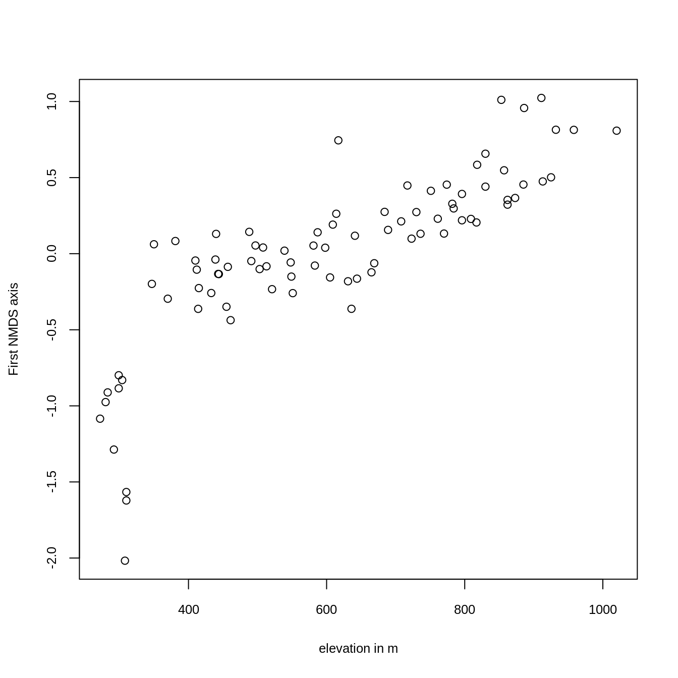

FIGURE 14.3: Plotting the first NMDS axis against altitude.

The scores of the first NMDS axis represent the different vegetation formations, i.e., the floristic gradient, appearing along the slope of Mt. Mongón. To spatially visualize them, we can model the NMDS scores with the previously created predictors (Section 14.2), and use the resulting model for predictive mapping (see next section).

14.4 Modeling the floristic gradient

To predict the floristic gradient spatially, we will make use of a random forest model (Hengl et al. 2018). Random forest models are frequently used in environmental and ecological modeling, and often provide the best results in terms of predictive performance (Schratz et al. 2018). Here, we shortly introduce decision trees and bagging, since they form the basis of random forests. We refer the reader to James et al. (2013) for a more detailed description of random forests and related techniques.

To introduce decision trees by example, we first construct a response-predictor matrix by joining the rotated NMDS scores to the field observations (random_points). We will also use the resulting data frame for the mlr modeling later on.

# construct response-predictor matrix
# id- and response variable
rp = data.frame(id = as.numeric(rownames(sc)), sc = sc[, 1])
# join the predictors (dem, ndvi and terrain attributes)
rp = inner_join(random_points, rp, by = "id")

Decision trees split the predictor space into a number of regions. To illustrate this, we apply a decision tree to our data using the scores of the first NMDS axis as the response (sc) and altitude (dem) as the only predictor.

library("tree")
tree_mo = tree(sc ~ dem, data = rp)
plot(tree_mo)
text(tree_mo, pretty = 0)

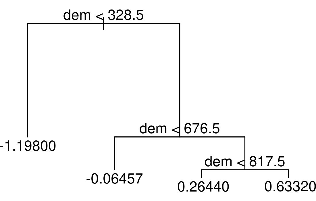
FIGURE 14.4: Simple example of a decision tree with three internal nodes and four terminal nodes.

The resulting tree consists of three internal nodes and four terminal nodes (Figure 14.4). The first internal node at the top of the tree assigns all observations which are below 328.5 to the left and all other observations to the right branch. The observations falling into the left branch have a mean NMDS score of -1.198. Overall, we can interpret the tree as follows: the higher the elevation, the higher the NMDS score becomes. Decision trees have a tendency to overfit, that is they mirror too closely the input data including its noise which in turn leads to bad predictive performances [Section 11.4; James et al. (2013)]. Bootstrap aggregation (bagging) is an ensemble technique and helps to overcome this problem. Ensemble techniques simply combine the predictions of multiple models. Thus, bagging takes repeated samples from the same input data and averages the predictions. This reduces the variance and overfitting with the result of a much better predictive accuracy compared to decision trees. Finally, random forests extend and improve bagging by decorrelating trees which is desirable since averaging the predictions of highly correlated trees shows a higher variance and thus lower reliability than averaging predictions of decorrelated trees (James et al. 2013). To achieve this, random forests use bagging, but in contrast to the traditional bagging where each tree is allowed to use all available predictors, random forests only use a random sample of all available predictors.

14.4.1 mlr building blocks

The code in this section largely follows the steps we have introduced in Section 11.5.2. The only differences are the following:

1. The response variable is numeric, hence a regression task will replace the classification task of Section 11.5.2.
2. Instead of the AUROC which can only be used for categorical response variables, we will use the root mean squared error (RMSE) as performance measure.
3. We use a random forest model instead of a support vector machine which naturally goes along with different hyperparameters.
4. We are leaving the assessment of a bias-reduced performance measure as an exercise to the reader (see Exercises). Instead we show how to tune hyperparameters for (spatial) predictions.

Remember that 125,500 models were necessary to retrieve bias-reduced performance estimates when using 100-repeated 5-fold spatial cross-validation and a random search of 50 iterations (see Section 11.5.2). In the hyperparameter tuning level, we found the best hyperparameter combination which in turn was used in the outer performance level for predicting the test data of a specific spatial partition (see also Figure 11.6). This was done for five spatial partitions, and repeated a 100 times yielding in total 500 optimal hyperparameter combinations. Which one should we use for making spatial predictions? The answer is simple, none at all. Remember, the tuning was done to retrieve a bias-reduced performance estimate, not to do the best possible spatial prediction. For the latter, one estimates the best hyperparameter combination from the complete dataset. This means, the inner hyperparameter tuning level is no longer needed which makes perfect sense since we are applying our model to new data (unvisited field observations) for which the true outcomes are unavailable, hence testing is impossible in any case. Therefore, we tune the hyperparameters for a good spatial prediction on the complete dataset via a 5-fold spatial CV with one repetition.

The preparation for the modeling using the mlr package includes the construction of a response-predictor matrix containing only variables which should be used in the modeling and the construction of a separate coordinate data frame.

# extract the coordinates into a separate data frame
coords = sf::st_coordinates(rp) %>% 
  as.data.frame() %>%
  rename(x = X, y = Y)
# only keep response and predictors which should be used for the modeling
rp = dplyr::select(rp, -id, -spri) %>%
  st_drop_geometry()

Having constructed the input variables, we are all set for specifying the mlr building blocks (task, learner, and resampling). We will use a regression task since the response variable is numeric. The learner is a random forest model implementation from the ranger package.

# create task
task = makeRegrTask(data = rp, target = "sc", coordinates = coords)
# learner
lrn_rf = makeLearner(cl = "regr.ranger", predict.type = "response")

As opposed to for example support vector machines (see Section 11.5.2), random forests often already show good performances when used with the default values of their hyperparameters (which may be one reason for their popularity). Still, tuning often moderately improves model results, and thus is worth the effort (Probst, Wright, and Boulesteix 2018). Since we deal with geographic data, we will again make use of spatial cross-validation to tune the hyperparameters (see Sections 11.4 and 11.5). Specifically, we will use a five-fold spatial partitioning with only one repetition (makeResampleDesc()). In each of these spatial partitions, we run 50 models (makeTuneControlRandom()) to find the optimal hyperparameter combination.

# spatial partitioning
perf_level = makeResampleDesc("SpCV", iters = 5)
# specifying random search
ctrl = makeTuneControlRandom(maxit = 50L)

In random forests, the hyperparameters mtry, min.node.size and sample.fraction determine the degree of randomness, and should be tuned (Probst, Wright, and Boulesteix 2018). mtry indicates how many predictor variables should be used in each tree. If all predictors are used, then this corresponds in fact to bagging (see beginning of Section 14.4). The sample.fraction parameter specifies the fraction of observations to be used in each tree. Smaller fractions lead to greater diversity, and thus less correlated trees which often is desirable (see above). The min.node.size parameter indicates the number of observations a terminal node should at least have (see also Figure 14.4). Naturally, as trees and computing time become larger, the lower the min.node.size.

Hyperparameter combinations will be selected randomly but should fall inside specific tuning limits (makeParamSet()). mtry should range between 1 and the number of predictors (4) sample.fraction should range between 0.2 and 0.9 and min.node.size should range between 1 and 10.

# specifying the search space
ps = makeParamSet(
  makeIntegerParam("mtry", lower = 1, upper = ncol(rp) - 1),
  makeNumericParam("sample.fraction", lower = 0.2, upper = 0.9),
  makeIntegerParam("min.node.size", lower = 1, upper = 10)
)

Finally, tuneParams() runs the hyperparameter tuning, and will find the optimal hyperparameter combination for the specified parameters. The performance measure is the root mean squared error (RMSE).

# hyperparamter tuning
set.seed(02082018)
tune = tuneParams(learner = lrn_rf, 
                  task = task,
                  resampling = perf_level,
                  par.set = ps,
                  control = ctrl, 
                  measures = mlr::rmse)
#>...
#> [Tune-x] 49: mtry=3; sample.fraction=0.533; min.node.size=5
#> [Tune-y] 49: rmse.test.rmse=0.5636692; time: 0.0 min
#> [Tune-x] 50: mtry=1; sample.fraction=0.68; min.node.size=5
#> [Tune-y] 50: rmse.test.rmse=0.6314249; time: 0.0 min
#> [Tune] Result: mtry=4; sample.fraction=0.887; min.node.size=10 :
#> rmse.test.rmse=0.5104918

An mtry of 4, a sample.fraction of 0.887, and a min.node.size of 10 represent the best hyperparameter combination. An RMSE of 0.51 is relatively good when considering the range of the response variable which is 3.04 (diff(range(rp$sc))).

14.4.2 Predictive mapping

The tuned hyperparameters can now be used for the prediction. We simply have to modify our learner using the result of the hyperparameter tuning, and run the corresponding model.

# learning using the best hyperparameter combination
lrn_rf = makeLearner(cl = "regr.ranger",
                     predict.type = "response",
                     mtry = tune$x$mtry, 
                     sample.fraction = tune$x$sample.fraction,
                     min.node.size = tune$x$min.node.size)
# doing the same more elegantly using setHyperPars()
# lrn_rf = setHyperPars(makeLearner("regr.ranger", predict.type = "response"),
#                       par.vals = tune$x)
# train model
model_rf = train(lrn_rf, task)
# to retrieve the ranger output, run:
# mlr::getLearnerModel(model_rf)
# which corresponds to:
# ranger(sc ~ ., data = rp, 
#        mtry = tune$x$mtry, 
#        sample.fraction = tune$x$sample.fraction,
#        min.node.sie = tune$x$min.node.size)

The last step is to apply the model to the spatially available predictors, i.e., to the raster stack. So far, raster::predict() does not support the output of ranger models, hence, we will have to program the prediction ourselves. First, we convert ep into a prediction data frame which secondly serves as input for the predict.ranger() function. Thirdly, we put the predicted values back into a RasterLayer (see Section 3.3.1 and Figure 14.5).

# convert raster stack into a data frame
new_data = as.data.frame(as.matrix(ep))
# apply the model to the data frame
pred_rf = predict(model_rf, newdata = new_data)
# put the predicted values into a raster
pred = dem
# replace altitudinal values by rf-prediction values
pred[] = pred_rf$data$response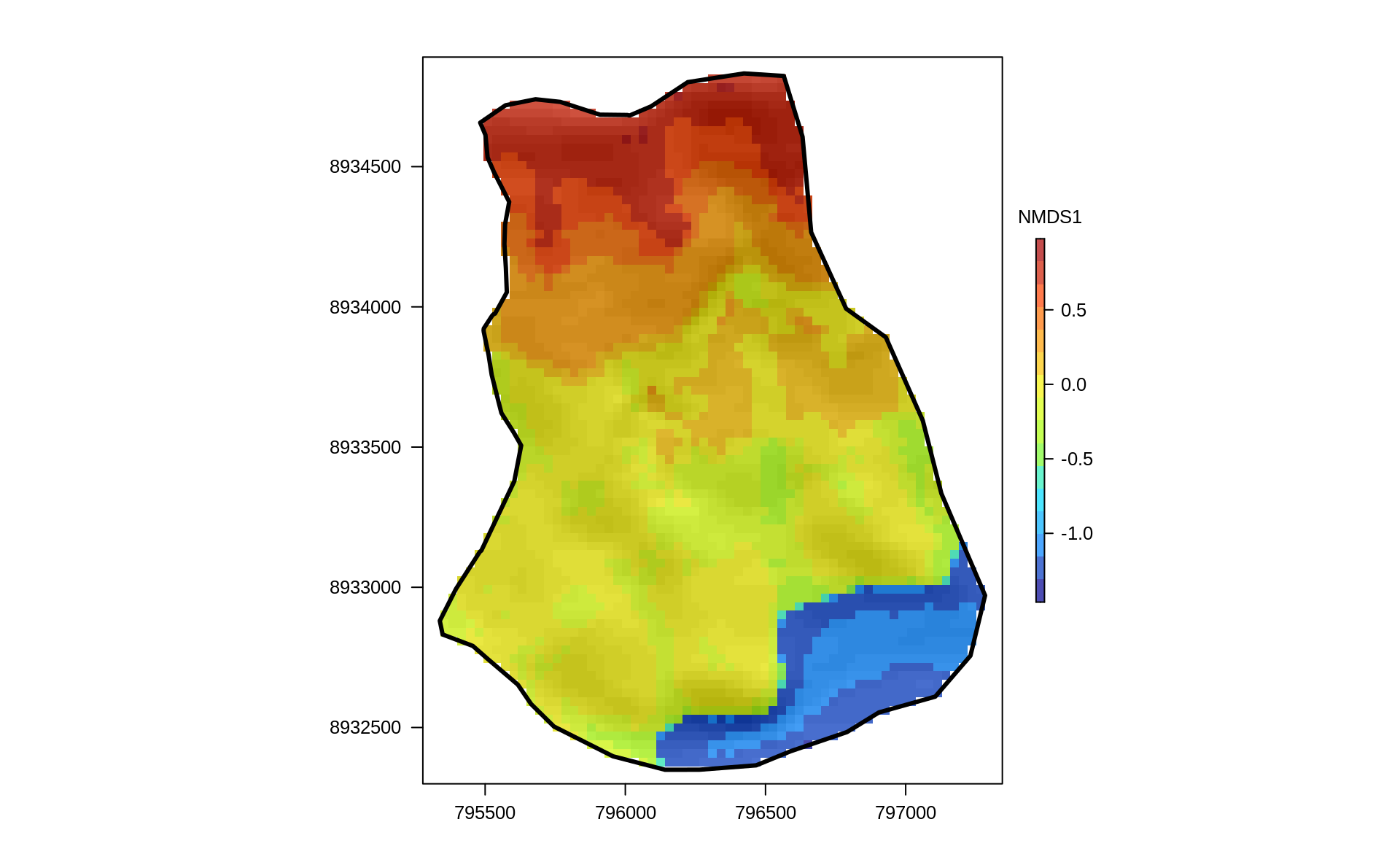

FIGURE 14.5: Predictive mapping of the floristic gradient clearly revealing distinct vegetation belts.

The predictive mapping clearly reveals distinct vegetation belts (Figure 14.5). Please refer to Muenchow, Hauenstein, et al. (2013) for a detailed description of vegetation belts on lomas mountains. The blue color tones represent the so-called Tillandsia-belt. Tillandsia is a highly adapted genus especially found in high quantities at the sandy and quite desertic foot of lomas mountains. The yellow color tones refer to a herbaceous vegetation belt with a much higher plant cover compared to the Tillandsia-belt. The orange colors represent the bromeliad belt, which features the highest species richness and plant cover. It can be found directly beneath the temperature inversion (ca. 750-850 m asl) where humidity due to fog is highest. Water availability naturally decreases above the temperature inversion, and the landscape becomes desertic again with only a few succulent species (succulent belt; red colors). Interestingly, the spatial prediction clearly reveals that the bromeliad belt is interrupted which is a very interesting finding we would have not detected without the predictive mapping.

14.5 Conclusions

In this chapter we have ordinated the community matrix of the lomas Mt. Mongón with the help of a NMDS (Section 14.3). The first axis, representing the main floristic gradient in the study area, was modeled as a function of environmental predictors which partly were derived through R-GIS bridges (Section 14.2). The mlr package provided the building blocks to spatially tune the hyperparameters mtry, sample.fraction and min.node.size (Section 14.4.1). The tuned hyperparameters served as input for the final model which in turn was applied to the environmental predictors for a spatial representation of the floristic gradient (Section 14.4.2). The result demonstrates spatially the astounding biodiversity in the middle of the desert. Since lomas mountains are heavily endangered, the prediction map can serve as basis for informed decision-making on delineating protection zones, and making the local population aware of the uniqueness found in their immediate neighborhood.

In terms of methodology, a few additional points could be addressed:

• It would be interesting to also model the second ordination axis, and to subsequently find an innovative way of visualizing jointly the modeled scores of the two axes in one prediction map.
• If we were interested in interpreting the model in an ecologically meaningful way, we should probably use (semi-)parametric models (Muenchow, Bräuning, et al. 2013; A. Zuur et al. 2009; A. F. Zuur et al. 2017). However, there are at least approaches that help to interpret machine learning models such as random forests (see, e.g., https://mlr-org.github.io/interpretable-machine-learning-iml-and-mlr/).
• A sequential model-based optimization (SMBO) might be preferable to the random search for hyperparameter optimization used in this chapter (Probst, Wright, and Boulesteix 2018).

Finally, please note that random forest and other machine learning models are frequently used in a setting with lots of observations and many predictors, much more than used in this chapter, and where it is unclear which variables and variable interactions contribute to explaining the response. Additionally, the relationships might be highly non-linear. In our use case, the relationship between response and predictors are pretty clear, there is only a slight amount of non-linearity and the number of observations and predictors is low. Hence, it might be worth trying a linear model. A linear model is much easier to explain and understand than a random forest model, and therefore to be preferred (law of parsimony), additionally it is computationally less demanding (see Exercises). If the linear model cannot cope with the degree of non-linearity present in the data, one could also try a generalized additive model (GAM). The point here is that the toolbox of a data scientist consists of more than one tool, and it is your responsibility to select the tool best suited for the task or purpose at hand. Here, we wanted to introduce the reader to random forest modeling and how to use the corresponding results for spatial predictions. For this purpose, a well-studied dataset with known relationships between response and predictors, is appropriate. However, this does not imply that the random forest model has returned the best result in terms of predictive performance (see Exercises).

14.6 Exercises

1. Run a NMDS using the percentage data of the community matrix. Report the stress value and compare it to the stress value as retrieved from the NMDS using presence-absence data. What might explain the observed difference?

2. Compute all the predictor rasters we have used in the chapter (catchment slope, catchment area), and put them into a raster stack. Add dem and ndvi to the raster stack. Next, compute profile and tangential curvature as additional predictor rasters and add them to the raster stack (hint: grass7:r.slope.aspect). Finally, construct a response-predictor matrix. The scores of the first NMDS axis (which were the result when using the presence-absence community matrix) rotated in accordance with elevation represent the response variable, and should be joined to random_points (use an inner join). To complete the response-predictor matrix, extract the values of the environmental predictor raster stack to random_points.

3. Use the response-predictor matrix of the previous exercise to fit a random forest model. Find the optimal hyperparameters and use them for making a prediction map.

4. Retrieve the bias-reduced RMSE of a random forest model using spatial cross-validation including the estimation of optimal hyperparameter combinations (random search with 50 iterations) in an inner tuning loop (see Section 11.5.2). Parallelize the tuning level (see Section 11.5.2). Report the mean RMSE and use a boxplot to visualize all retrieved RMSEs.

5. Retrieve the bias-reduced RMSE of a simple linear model using spatial cross-validation. Compare the result to the result of the random forest model by making RMSE boxplots for each modeling approach.