6 Reprojecting geographic data

Prerequisites

• This chapter requires the following packages (lwgeom is also used, but does not need to be attached):

library(sf)
library(terra)
library(dplyr)
library(spData)
library(spDataLarge)

6.1 Introduction

Section 2.4 introduced coordinate reference systems (CRSs) and demonstrated their importance. This chapter goes further. It highlights issues that can arise when using inappropriate CRSs and how to transform data from one CRS to another.

As illustrated in Figure 2.1, there are two types of CRSs: geographic (‘lon/lat,’ with units in degrees longitude and latitude) and projected (typically with units of meters from a datum). This has consequences. Many geometry operations in sf, for example, assume their inputs have a projected CRS, because the GEOS functions they are based on assume projected data. To deal with this issue sf provides the function st_is_longlat() to check. In some cases the CRS is unknown, as shown below using the example of London introduced in Section 2.2:

london = data.frame(lon = -0.1, lat = 51.5) %>% 
  st_as_sf(coords = c("lon", "lat"))
st_is_longlat(london)
#> [1] NA

This shows that unless a CRS is manually specified or is loaded from a source that has CRS metadata, the CRS is NA. A CRS can be added to sf objects with st_set_crs() as follows:²⁷

london_geo = st_set_crs(london, 4326)
st_is_longlat(london_geo)
#> [1] TRUE

Datasets without a specified CRS can cause problems. An example is provided below, which creates a buffer of one unit around london and london_geo objects:

london_buff_no_crs = st_buffer(london, dist = 1)
london_buff = st_buffer(london_geo, dist = 1)

Only the second operation generates a warning. The warning message is useful, telling us that the result may be of limited use because it is in units of latitude and longitude, rather than meters or some other suitable measure of distance assumed by st_buffer(). The consequences of a failure to work on projected data are illustrated in Figure 6.1 (left panel): the buffer is elongated in the north-south direction because lines of longitude converge towards the Earth’s poles.

The distance between two lines of longitude, called meridians, is around 111 km at the equator (execute geosphere::distGeo(c(0, 0), c(1, 0)) to find the precise distance). This shrinks to zero at the poles. At the latitude of London, for example, meridians are less than 70 km apart (challenge: execute code that verifies this). Lines of latitude, by contrast, are equidistant from each other irrespective of latitude: they are always around 111 km apart, including at the equator and near the poles (see Figures 6.1 to 6.3).

Do not interpret the warning about the geographic (longitude/latitude) CRS as “the CRS should not be set”: it almost always should be! It is better understood as a suggestion to reproject the data onto a projected CRS. This suggestion does not always need to be heeded: performing spatial and geometric operations makes little or no difference in some cases (e.g., spatial subsetting). But for operations involving distances such as buffering, the only way to ensure a good result is to create a projected copy of the data and run the operation on that. This is done in the code chunk below:

london_proj = data.frame(x = 530000, y = 180000) %>% 
  st_as_sf(coords = 1:2, crs = 27700)

The result is a new object that is identical to london, but reprojected onto a suitable CRS (the British National Grid, which has an EPSG code of 27700 in this case) that has units of meters. We can verify that the CRS has changed using st_crs() as follows (some of the output has been replaced by ...):

st_crs(london_proj)
#> Coordinate Reference System:
#>   EPSG: 27700 
#>   proj4string: "+proj=tmerc +lat_0=49 +lon_0=-2 ... +units=m +no_defs"

Notable components of this CRS description include the EPSG code (EPSG: 27700), the projection (transverse Mercator, +proj=tmerc), the origin (+lat_0=49 +lon_0=-2) and units (+units=m).²⁸ The fact that the units of the CRS are meters (rather than degrees) tells us that this is a projected CRS: st_is_longlat(london_proj) now returns FALSE and geometry operations on london_proj will work without a warning, meaning buffers can be produced from it using proper units of distance. As pointed out above, moving one degree means moving a bit more than 111 km at the equator (to be precise: 111,320 meters). This is used as the new buffer distance:

london_proj_buff = st_buffer(london_proj, 111320)

The result in Figure 6.1 (right panel) shows that buffers based on a projected CRS are not distorted: every part of the buffer’s border is equidistant to London.

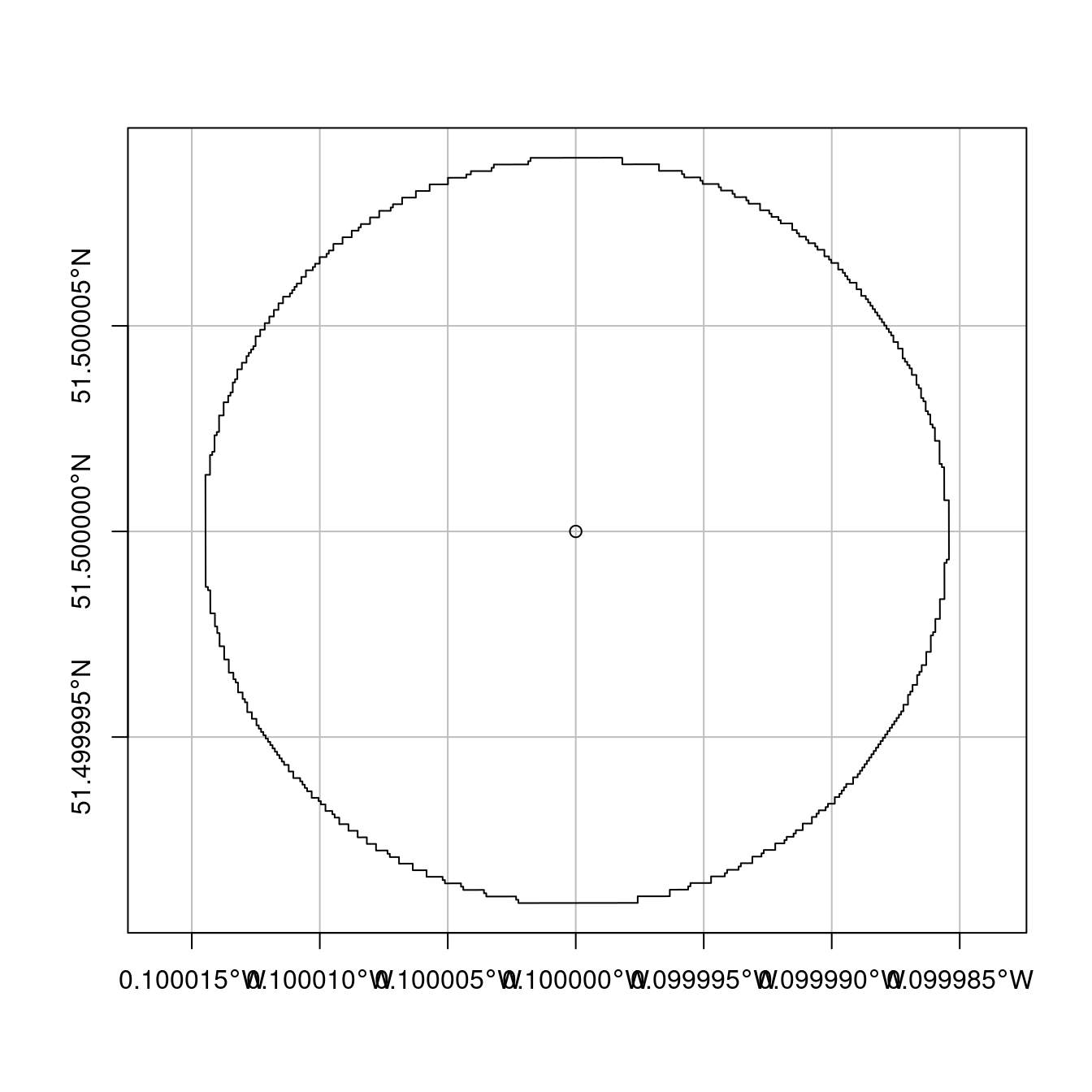
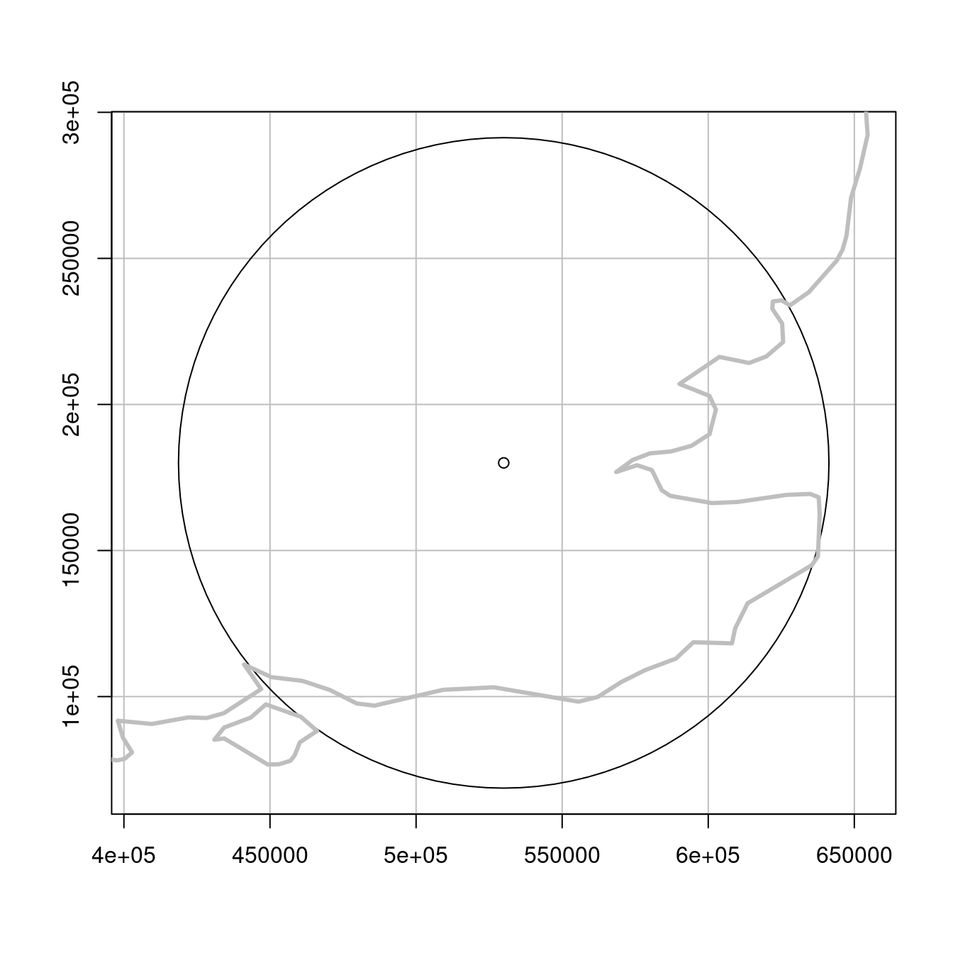
FIGURE 6.1: Buffers around London with a geographic (left) and projected (right) CRS. The gray outline represents the UK coastline.

The importance of CRSs (primarily whether they are projected or geographic) has been demonstrated using the example of London. The subsequent sections go into more depth, exploring which CRS to use and the details of reprojecting vector and raster objects.

6.2 When to reproject?

The previous section showed how to set the CRS manually, with st_set_crs(london, 4326). In real world applications, however, CRSs are usually set automatically when data is read-in. The main task involving CRSs is often to transform objects, from one CRS into another. But when should data be transformed? And into which CRS? There are no clear-cut answers to these questions and CRS selection always involves trade-offs (Maling 1992). However, there are some general principles provided in this section that can help you decide.

First it’s worth considering when to transform. In some cases transformation to a projected CRS is essential, such as when using geometric functions such as st_buffer(), as Figure 6.1 showed. Conversely, publishing data online with the leaflet package may require a geographic CRS. Another case is when two objects with different CRSs must be compared or combined, as shown when we try to find the distance between two objects with different CRSs:

st_distance(london_geo, london_proj)
# > Error: st_crs(x) == st_crs(y) is not TRUE

To make the london and london_proj objects geographically comparable one of them must be transformed into the CRS of the other. But which CRS to use? The answer is usually ‘to the projected CRS,’ which in this case is the British National Grid (EPSG:27700):

london2 = st_transform(london_geo, 27700)

Now that a transformed version of london has been created, using the sf function st_transform(), the distance between the two representations of London can be found. It may come as a surprise that london and london2 are just over 2 km apart!²⁹

st_distance(london2, london_proj)
#> Units: [m]
#>      [,1]
#> [1,] 2018

6.3 Which CRS to use?

The question of which CRS is tricky, and there is rarely a ‘right’ answer: “There exist no all-purpose projections, all involve distortion when far from the center of the specified frame” (R. Bivand, Pebesma, and Gómez-Rubio 2013).

For geographic CRSs, the answer is often WGS84, not only for web mapping, but also because GPS datasets and thousands of raster and vector datasets are provided in this CRS by default. WGS84 is the most common CRS in the world, so it is worth knowing its EPSG code: 4326. This ‘magic number’ can be used to convert objects with unusual projected CRSs into something that is widely understood.

What about when a projected CRS is required? In some cases, it is not something that we are free to decide: “often the choice of projection is made by a public mapping agency” (R. Bivand, Pebesma, and Gómez-Rubio 2013). This means that when working with local data sources, it is likely preferable to work with the CRS in which the data was provided, to ensure compatibility, even if the official CRS is not the most accurate. The example of London was easy to answer because (a) the British National Grid (with its associated EPSG code 27700) is well known and (b) the original dataset (london) already had that CRS.

In cases where an appropriate CRS is not immediately clear, the choice of CRS should depend on the properties that are most important to preserve in the subsequent maps and analysis. All CRSs are either equal-area, equidistant, conformal (with shapes remaining unchanged), or some combination of compromises of those. Custom CRSs with local parameters can be created for a region of interest and multiple CRSs can be used in projects when no single CRS suits all tasks. ‘Geodesic calculations’ can provide a fall-back if no CRSs are appropriate (see proj.org/geodesic.html). Regardless of the projected CRS used, the results may not be accurate for geometries covering hundreds of kilometers.

When deciding on a custom CRS, we recommend the following:³⁰

• A Lambert azimuthal equal-area (LAEA) projection for a custom local projection (set lon_0 and lat_0 to the center of the study area), which is an equal-area projection at all locations but distorts shapes beyond thousands of kilometres
• Azimuthal equidistant (AEQD) projections for a specifically accurate straight-line distance between a point and the centre point of the local projection
• Lambert conformal conic (LCC) projections for regions covering thousands of kilometres, with the cone set to keep distance and area properties reasonable between the secant lines
• Stereographic (STERE) projections for polar regions, but taking care not to rely on area and distance calculations thousands of kilometres from the center

A commonly used default is Universal Transverse Mercator (UTM), a set of CRSs that divides the Earth into 60 longitudinal wedges and 20 latitudinal segments. The transverse Mercator projection used by UTM CRSs is conformal but distorts areas and distances with increasing severity with distance from the center of the UTM zone. Documentation from the GIS software Manifold therefore suggests restricting the longitudinal extent of projects using UTM zones to 6 degrees from the central meridian (source: manifold.net).

Almost every place on Earth has a UTM code, such as “60H” which refers to northern New Zealand where R was invented. UTM EPSG codes run sequentially from 32601 to 32660 for northern hemisphere locations and from 32701 to 32760 for southern hemisphere locations.

To show how the system works, let’s create a function, lonlat2UTM() to calculate the EPSG code associated with any point on the planet as follows:

lonlat2UTM = function(lonlat) {
  utm = (floor((lonlat[1] + 180) / 6) %% 60) + 1
  if(lonlat[2] > 0) {
    utm + 32600
  } else{
    utm + 32700
  }
}

The following command uses this function to identify the UTM zone and associated EPSG code for Auckland and London:

epsg_utm_auk = lonlat2UTM(c(174.7, -36.9))
epsg_utm_lnd = lonlat2UTM(st_coordinates(london))
st_crs(epsg_utm_auk)$proj4string
#> [1] "+proj=utm +zone=60 +south +datum=WGS84 +units=m +no_defs"
st_crs(epsg_utm_lnd)$proj4string
#> [1] "+proj=utm +zone=30 +datum=WGS84 +units=m +no_defs"

Maps of UTM zones such as that provided by dmap.co.uk confirm that London is in UTM zone 30U.

Another approach to automatically select a projected CRS specific to a local dataset is to create an azimuthal equidistant (AEQD) projection for the center-point of the study area. This involves creating a custom CRS (with no EPSG code) with units of meters based on the centerpoint of a dataset. This approach should be used with caution: no other datasets will be compatible with the custom CRS created and results may not be accurate when used on extensive datasets covering hundreds of kilometers.

The principles outlined in this section apply equally to vector and raster datasets. Some features of CRS transformation however are unique to each geographic data model. We will cover the particularities of vector data transformation in Section 6.4 and those of raster transformation in Section 6.6.

6.4 Reprojecting vector geometries

Chapter 2 demonstrated how vector geometries are made-up of points, and how points form the basis of more complex objects such as lines and polygons. Reprojecting vectors thus consists of transforming the coordinates of these points. This is illustrated by cycle_hire_osm, an sf object from spData that represents cycle hire locations across London. The previous section showed how the CRS of vector data can be queried with st_crs(). Although the output of this function is printed as a single entity, the result is in fact a named list of class crs, with names proj4string (which contains full details of the CRS) and epsg for its code. This is demonstrated below:

crs_lnd = st_crs(cycle_hire_osm)
class(crs_lnd)
#> [1] "crs"
crs_lnd$epsg
#> [1] 4326

This duality of CRS objects means that they can be set either using an EPSG code or a proj4string. This means that st_crs("+proj=longlat +datum=WGS84 +no_defs") is equivalent to st_crs(4326), although not all proj4strings have an associated EPSG code. Both elements of the CRS are changed by transforming the object to a projected CRS:

cycle_hire_osm_projected = st_transform(cycle_hire_osm, 27700)

The resulting object has a new CRS with an EPSG code 27700. But how to find out more details about this EPSG code, or any code? One option is to search for it online. Another option is to use a function from the rgdal package to find the name of the CRS:

crs_codes = rgdal::make_EPSG()[1:2]
dplyr::filter(crs_codes, code == 27700)
#>    code                              note
#> 1 27700 OSGB 1936 / British National Grid

The result shows that the EPSG code 27700 represents the British National Grid, a result that could have been found by searching online for “EPSG 27700.” But what about the proj4string element? proj4strings are text strings that describe the CRS. They can be seen as formulas for converting a projected point into a point on the surface of the Earth and can be accessed from crs objects as follows (see proj.org/ for further details of what the output means):

st_crs(27700)$proj4string
#> [1] "+proj=tmerc +lat_0=49 +lon_0=-2 +k=0.9996012717 +x_0=400000 ...

Printing a spatial object in the console automatically returns its coordinate reference system. To access and modify it explicitly, use the st_crs function, for example, st_crs(cycle_hire_osm).

6.5 Modifying map projections

Established CRSs captured by EPSG codes are well-suited for many applications. However in some cases it is desirable to create a new CRS, using a custom proj4string. This system allows a very wide range of projections to be created, as we’ll see in some of the custom map projections in this section.

A long and growing list of projections has been developed and many of these can be set with the +proj= element of proj4strings.³¹

When mapping the world while preserving area relationships, the Mollweide projection is a good choice (Jenny et al. 2017) (Figure 6.2). To use this projection, we need to specify it using the proj4string element, "+proj=moll", in the st_transform function:

world_mollweide = st_transform(world, crs = "+proj=moll")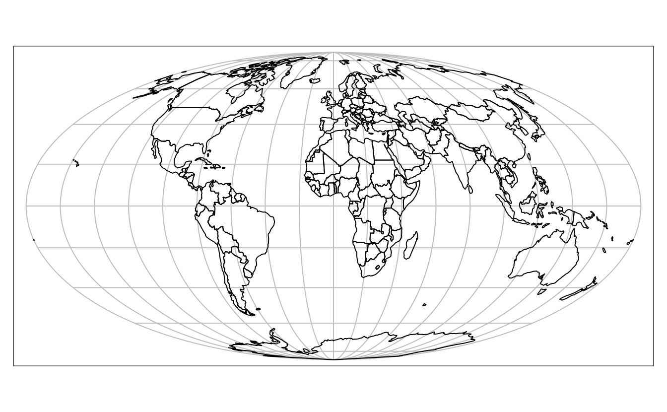

FIGURE 6.2: Mollweide projection of the world.

On the other hand, when mapping the world, it is often desirable to have as little distortion as possible for all spatial properties (area, direction, distance). One of the most popular projections to achieve this is the Winkel tripel projection (Figure 6.3).³² st_transform_proj() from the lwgeom package allows for coordinate transformations to a wide range of CRSs, including the Winkel tripel projection:

world_wintri = lwgeom::st_transform_proj(world, crs = "+proj=wintri")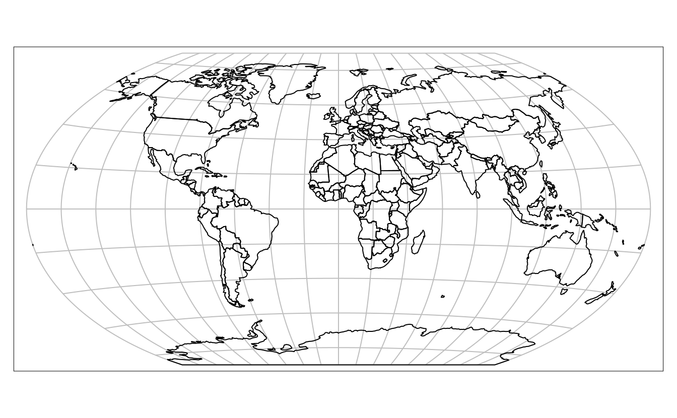

FIGURE 6.3: Winkel tripel projection of the world.

The three main functions for transformation of simple features coordinates are sf::st_transform(), sf::sf_project(), and lwgeom::st_transform_proj(). The st_transform function uses the GDAL interface to PROJ, while sf_project() (which works with two-column numeric matrices, representing points) and lwgeom::st_transform_proj() use the PROJ API directly. The first one is appropriate for most situations, and provides a set of the most often used parameters and well-defined transformations. The next one allows for greater customization of a projection, which includes cases when some of the PROJ parameters (e.g., +over) or projection (+proj=wintri) is not available in st_transform().

Moreover, PROJ parameters can be modified in most CRS definitions. The below code transforms the coordinates to the Lambert azimuthal equal-area projection centered on longitude and latitude of 0 (Figure 6.4).

world_laea1 = st_transform(world, 
                           crs = "+proj=laea +x_0=0 +y_0=0 +lon_0=0 +lat_0=0")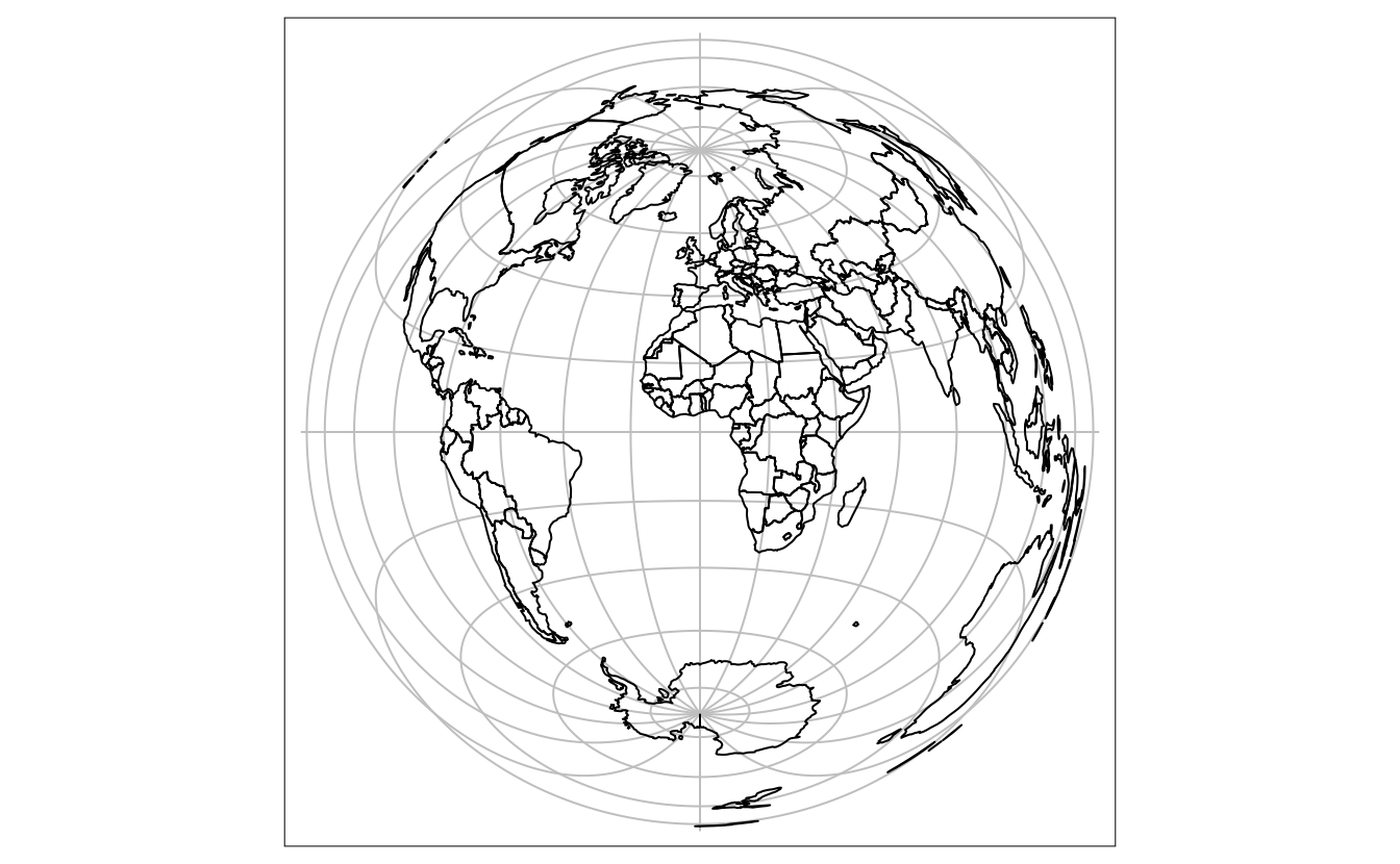

FIGURE 6.4: Lambert azimuthal equal-area projection centered on longitude and latitude of 0.

We can change the PROJ parameters, for example the center of the projection, using the +lon_0 and +lat_0 parameters. The code below gives the map centered on New York City (Figure 6.5).

world_laea2 = st_transform(world,
                           crs = "+proj=laea +x_0=0 +y_0=0 +lon_0=-74 +lat_0=40")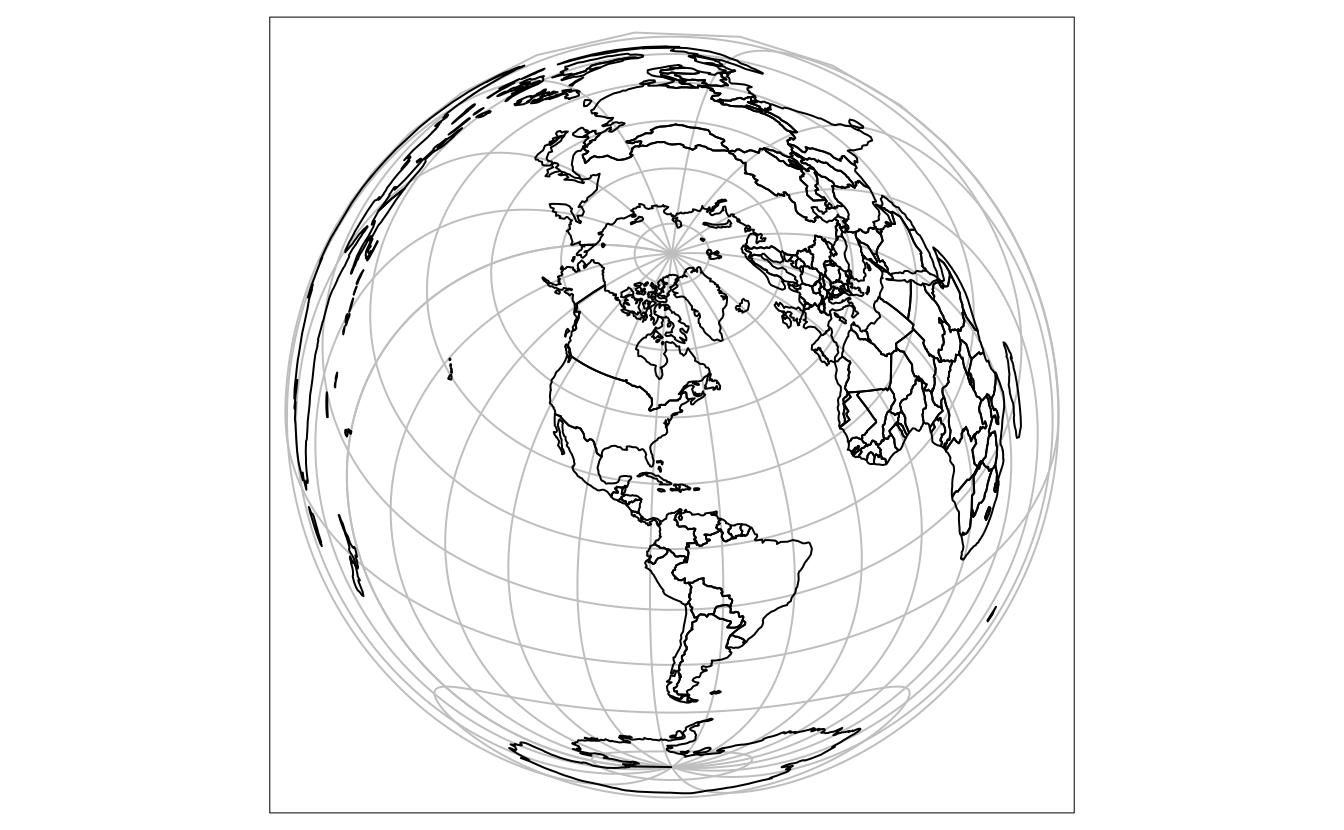

FIGURE 6.5: Lambert azimuthal equal-area projection of the world centered on New York City.

More information on CRS modifications can be found in the Using PROJ documentation.

6.6 Reprojecting raster geometries

The projection concepts described in the previous section apply equally to rasters. However, there are important differences in reprojection of vectors and rasters: transforming a vector object involves changing the coordinates of every vertex but this does not apply to raster data. Rasters are composed of rectangular cells of the same size (expressed by map units, such as degrees or meters), so it is usually impracticable to transform coordinates of pixels separately. Raster reprojection involves creating a new raster object, often with a different number of columns and rows than the original. The attributes must subsequently be re-estimated, allowing the new pixels to be ‘filled’ with appropriate values. In other words, raster reprojection can be thought of as two separate spatial operations: a vector reprojection of the raster extent to another CRS (Section 6.4), and computation of new pixel values through resampling (Section 5.3.4). Thus in most cases when both raster and vector data are used, it is better to avoid reprojecting rasters and reproject vectors instead.

Reprojection of the regular rasters is also known as warping. Additionally, there is a second similar operation called “transformation.” Instead of resampling all of the values, it leaves all values intact but recomputes new coordinates for every raster cell, changing the grid geometry. For example, it could convert the input raster (a regular grid) into a curvilinear grid. The transformation operation can be performed in R using the stars package.

The raster reprojection process is done with project() from the terra package. Like the st_transform() function demonstrated in the previous section, project() takes a geographic object (a raster dataset in this case) and some CRS representation as the second argument. On a side note – the second argument can also be an existing raster object with a different CRS.

Let’s take a look at two examples of raster transformation: using categorical and continuous data. Land cover data are usually represented by categorical maps. The nlcd.tif file provides information for a small area in Utah, USA obtained from National Land Cover Database 2011 in the NAD83 / UTM zone 12N CRS.

cat_raster = rast(system.file("raster/nlcd.tif", package = "spDataLarge"))
crs(cat_raster)
#> [1] "PROJCRS[\"NAD83 / UTM zone 12N\",\n    BASEGEOGCRS[\"NAD83\",\n        DATUM[\"North American Datum 1983\",\n            ELLIPSOID[\"GRS 1980\",6378137,298.257222101,\n                LENGTHUNIT[\"metre\",1]]],\n        PRIMEM[\"Greenwich\",0,\n            ANGLEUNIT[\"degree\",0.0174532925199433]],\n        ID[\"EPSG\",4269]],\n    CONVERSION[\"UTM zone 12N\",\n        METHOD[\"Transverse Mercator\",\n            ID[\"EPSG\",9807]],\n        PARAMETER[\"Latitude of natural origin\",0,\n            ANGLEUNIT[\"degree\",0.0174532925199433],\n            ID[\"EPSG\",8801]],\n        PARAMETER[\"Longitude of natural origin\",-111,\n            ANGLEUNIT[\"degree\",0.0174532925199433],\n            ID[\"EPSG\",8802]],\n        PARAMETER[\"Scale factor at natural origin\",0.9996,\n            SCALEUNIT[\"unity\",1],\n            ID[\"EPSG\",8805]],\n        PARAMETER[\"False easting\",500000,\n            LENGTHUNIT[\"metre\",1],\n            ID[\"EPSG\",8806]],\n        PARAMETER[\"False northing\",0,\n            LENGTHUNIT[\"metre\",1],\n            ID[\"EPSG\",8807]]],\n    CS[Cartesian,2],\n        AXIS[\"(E)\",east,\n            ORDER[1],\n            LENGTHUNIT[\"metre\",1]],\n        AXIS[\"(N)\",north,\n            ORDER[2],\n            LENGTHUNIT[\"metre\",1]],\n    USAGE[\n        SCOPE[\"unknown\"],\n        AREA[\"North America - 114°W to 108°W and NAD83 by country\"],\n        BBOX[31.33,-114,84,-108]],\n    ID[\"EPSG\",26912]]"

In this region, 8 land cover classes were distinguished (a full list of NLCD2011 land cover classes can be found at mrlc.gov):

unique(cat_raster)
#>   levels
#> 1      1
#> 2      2
#> 3      3
#> 4      4
#> 5      5
#> 6      6
#> 7      7
#> 8      8

When reprojecting categorical rasters, the estimated values must be the same as those of the original. This could be done using the nearest neighbor method (near), which sets each new cell value to the value of the nearest cell (center) of the input raster. An example is reprojecting cat_raster to WGS84, a geographic CRS well suited for web mapping. The first step is to obtain the PROJ definition of this CRS, which can be done, for example using the http://spatialreference.org webpage. The final step is to reproject the raster with the project() function which, in the case of categorical data, uses the nearest neighbor method (near):

cat_raster_wgs84 = project(cat_raster, "EPSG:4326", method = "near")

Many properties of the new object differ from the previous one, including the number of columns and rows (and therefore number of cells), resolution (transformed from meters into degrees), and extent, as illustrated in Table 6.1 (note that the number of categories increases from 8 to 9 because of the addition of NA values, not because a new category has been created — the land cover classes are preserved).

TABLE 6.1: Key attributes in the original (‘cat_raster’) and projected (‘cat_raster_wgs84’) categorical raster datasets.

CRS	nrow	ncol	ncell	resolution	unique_categories
NAD83	1359	1073	1458207	31.5275	8
WGS84	1246	1244	1550024	0.0003	9

Reprojecting numeric rasters (with numeric or in this case integer values) follows an almost identical procedure. This is demonstrated below with srtm.tif in spDataLarge from the Shuttle Radar Topography Mission (SRTM), which represents height in meters above sea level (elevation) with the WGS84 CRS:

con_raster = rast(system.file("raster/srtm.tif", package = "spDataLarge"))
crs(con_raster)
#> [1] "GEOGCRS[\"WGS 84\",\n    DATUM[\"World Geodetic System 1984\",\n        ELLIPSOID[\"WGS 84\",6378137,298.257223563,\n            LENGTHUNIT[\"metre\",1]]],\n    PRIMEM[\"Greenwich\",0,\n        ANGLEUNIT[\"degree\",0.0174532925199433]],\n    CS[ellipsoidal,2],\n        AXIS[\"geodetic latitude (Lat)\",north,\n            ORDER[1],\n            ANGLEUNIT[\"degree\",0.0174532925199433]],\n        AXIS[\"geodetic longitude (Lon)\",east,\n            ORDER[2],\n            ANGLEUNIT[\"degree\",0.0174532925199433]],\n    ID[\"EPSG\",4326]]"

We will reproject this dataset into a projected CRS, but not with the nearest neighbor method which is appropriate for categorical data. Instead, we will use the bilinear method which computes the output cell value based on the four nearest cells in the original raster.³³ The values in the projected dataset are the distance-weighted average of the values from these four cells: the closer the input cell is to the center of the output cell, the greater its weight. The following commands create a text string representing WGS 84 / UTM zone 12N, and reproject the raster into this CRS, using the bilinear method:

con_raster_ea = project(con_raster, "EPSG:32612", method = "bilinear")
crs(con_raster_ea)
#> [1] "PROJCRS[\"WGS 84 / UTM zone 12N\",\n    BASEGEOGCRS[\"WGS 84\",\n        DATUM[\"World Geodetic System 1984\",\n            ELLIPSOID[\"WGS 84\",6378137,298.257223563,\n                LENGTHUNIT[\"metre\",1]]],\n        PRIMEM[\"Greenwich\",0,\n            ANGLEUNIT[\"degree\",0.0174532925199433]],\n        ID[\"EPSG\",4326]],\n    CONVERSION[\"UTM zone 12N\",\n        METHOD[\"Transverse Mercator\",\n            ID[\"EPSG\",9807]],\n        PARAMETER[\"Latitude of natural origin\",0,\n            ANGLEUNIT[\"degree\",0.0174532925199433],\n            ID[\"EPSG\",8801]],\n        PARAMETER[\"Longitude of natural origin\",-111,\n            ANGLEUNIT[\"degree\",0.0174532925199433],\n            ID[\"EPSG\",8802]],\n        PARAMETER[\"Scale factor at natural origin\",0.9996,\n            SCALEUNIT[\"unity\",1],\n            ID[\"EPSG\",8805]],\n        PARAMETER[\"False easting\",500000,\n            LENGTHUNIT[\"metre\",1],\n            ID[\"EPSG\",8806]],\n        PARAMETER[\"False northing\",0,\n            LENGTHUNIT[\"metre\",1],\n            ID[\"EPSG\",8807]]],\n    CS[Cartesian,2],\n        AXIS[\"(E)\",east,\n            ORDER[1],\n            LENGTHUNIT[\"metre\",1]],\n        AXIS[\"(N)\",north,\n            ORDER[2],\n            LENGTHUNIT[\"metre\",1]],\n    USAGE[\n        SCOPE[\"unknown\"],\n        AREA[\"World - N hemisphere - 114°W to 108°W - by country\"],\n        BBOX[0,-114,84,-108]],\n    ID[\"EPSG\",32612]]"

Raster reprojection on numeric variables also leads to small changes to values and spatial properties, such as the number of cells, resolution, and extent. These changes are demonstrated in Table 6.2³⁴:

TABLE 6.2: Key attributes in the original (‘con_raster’) and projected (‘con_raster_ea’) continuous raster datasets.

CRS	nrow	ncol	ncell	resolution	mean
WGS84	457	465	212505	0.0008	1843
UTM zone 12N	515	422	217330	83.5334	1842

Of course, the limitations of 2D Earth projections apply as much to vector as to raster data. At best we can comply with two out of three spatial properties (distance, area, direction). Therefore, the task at hand determines which projection to choose. For instance, if we are interested in a density (points per grid cell or inhabitants per grid cell) we should use an equal-area projection (see also Chapter 13).

There is more to learn about CRSs. An excellent resource in this area, also implemented in R, is the website R Spatial. Chapter 6 for this free online book is recommended reading — see: rspatial.org/terra/spatial/6-crs.html

6.7 Exercises

E1. Create a new object called nz_wgs by transforming nz object into the WGS84 CRS.

• Create an object of class crs for both and use this to query their CRSs.
• With reference to the bounding box of each object, what units does each CRS use?
• Remove the CRS from nz_wgs and plot the result: what is wrong with this map of New Zealand and why?

E2. Transform the world dataset to the transverse Mercator projection ("+proj=tmerc") and plot the result. What has changed and why? Try to transform it back into WGS 84 and plot the new object. Why does the new object differ from the original one?

E3. Transform the continuous raster (con_raster) into NAD83 / UTM zone 12N using the nearest neighbor interpolation method. What has changed? How does it influence the results?

E4. Transform the categorical raster (cat_raster) into WGS 84 using the bilinear interpolation method. What has changed? How does it influence the results?

E5. Create your own proj4string. It should have the Lambert Azimuthal Equal Area (laea) projection, the WGS84 ellipsoid, the longitude of projection center of 95 degrees west, the latitude of projection center of 60 degrees north, and its units should be in meters. Next, subset Canada from the world object and transform it into the new projection. Plot and compare a map before and after the transformation.