10 Scripts, algorithms and functions

Prerequisites

This chapter primarily uses base R; the sf package is used to check the result of an algorithm we will develop. It assumes you have an understanding of the geographic classes introduced in Chapter 2 and how they can be used to represent a wide range of input file formats (see Chapter 7).

10.1 Introduction

Chapter 1 established that geocomputation is not only about using existing tools, but developing new ones, “in the form of shareable R scripts and functions.” This chapter teaches these building blocks of reproducible code. It also introduces low-level geometric algorithms, of the type used in Chapter 9. Reading it should help you to understand how such algorithms work and to write code that can be used many times, by many people, on multiple datasets. The chapter cannot, by itself, make you a skilled programmer. Programming is hard and requires plenty of practice (Abelson, Sussman, and Sussman 1996):

To appreciate programming as an intellectual activity in its own right you must turn to computer programming; you must read and write computer programs — many of them.

There are strong reasons for moving in that direction, however.⁵⁷ The advantages of reproducibility go beyond allowing others to replicate your work: reproducible code is often better in every way than code written to be run only once, including in terms of computational efficiency, scalability and ease of adapting and maintaining it.

Scripts are the basis of reproducible R code, a topic covered in Section 10.2. Algorithms are recipes for modifying inputs using a series of steps, resulting in an output, as described in Section 10.3. To ease sharing and reproducibility, algorithms can be placed into functions. That is the topic of Section 10.4. The example of finding the centroid of a polygon will be used to tie these concepts together. Chapter 5 already introduced a centroid function st_centroid(), but this example highlights how seemingly simple operations are the result of comparatively complex code, affirming the following observation (Wise 2001):

One of the most intriguing things about spatial data problems is that things which appear to be trivially easy to a human being can be surprisingly difficult on a computer.

The example also reflects a secondary aim of the chapter which, following Xiao (2016), is “not to duplicate what is available out there, but to show how things out there work.”

10.2 Scripts

If functions distributed in packages are the building blocks of R code, scripts are the glue that holds them together, in a logical order, to create reproducible workflows. To programming novices scripts may sound intimidating but they are simply plain text files, typically saved with an extension representing the language they contain. R scripts are generally saved with a .R extension and named to reflect what they do. An example is 10-hello.R, a script file stored in the code folder of the book’s repository, which contains the following two lines of code:

# Aim: provide a minimal R script
print("Hello geocompr")

The lines of code may not be particularly exciting but they demonstrate the point: scripts do not need to be complicated. Saved scripts can be called and executed in their entirety with source(), as demonstrated below which shows how the comment is ignored but the instruction is executed:

source("code/10-hello.R")
#> [1] "Hello geocompr"

There are no strict rules on what can and cannot go into script files and nothing to prevent you from saving broken, non-reproducible code.⁵⁸ There are, however, some conventions worth following:

• Write the script in order: just like the script of a film, scripts should have a clear order such as ‘setup,’ ‘data processing’ and ‘save results’ (roughly equivalent to ‘beginning,’ ‘middle’ and ‘end’ in a film).

• Add comments to the script so other people (and your future self) can understand it. At a minimum, a comment should state the purpose of the script (see Figure 10.1) and (for long scripts) divide it into sections. This can be done in RStudio, for example, with the shortcut Ctrl+Shift+R, which creates ‘foldable’ code section headings.

• Above all, scripts should be reproducible: self-contained scripts that will work on any computer are more useful than scripts that only run on your computer, on a good day. This involves attaching required packages at the beginning, reading-in data from persistent sources (such as a reliable website) and ensuring that previous steps have been taken.⁵⁹

It is hard to enforce reproducibility in R scripts, but there are tools that can help. By default, RStudio ‘code-checks’ R scripts and underlines faulty code with a red wavy line, as illustrated below:

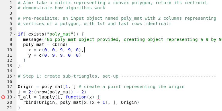
FIGURE 10.1: Code checking in RStudio. This example, from the script 10-centroid-alg.R, highlights an unclosed curly bracket on line 19.

A useful tool for reproducibility is the reprex package. Its main function reprex() tests lines of R code to check if they are reproducible, and provides markdown output to facilitate communication on sites such as GitHub. See the web page reprex.tidyverse.org for details.

The contents of this section apply to any type of R script. A particular consideration with scripts for geocomputation is that they tend to have external dependencies, such as the QGIS dependency to run code in Chapter 9, and require input data in a specific format. Such dependencies should be mentioned as comments in the script or elsewhere in the project of which it is a part, as illustrated in the script 10-centroid-alg.R. The work undertaken by this script is demonstrated in the reproducible example below, which works on a pre-requisite object named poly_mat, a square with sides 9 units in length (the meaning of this will become apparent in the next section):⁶⁰

poly_mat = cbind(
  x = c(0, 0, 9, 9, 0),
  y = c(0, 9, 9, 0, 0)
)
source("https://git.io/10-centroid-alg.R") # short url

#> [1] "The area is: 81"
#> [1] "The coordinates of the centroid are: 4.5, 4.5"

10.3 Geometric algorithms

Algorithms can be understood as the computing equivalent of a cooking recipe. They are a complete set of instructions which, when undertaken on the input (ingredients), result in useful (tasty) outputs. Before diving into a concrete case study, a brief history will show how algorithms relate to scripts (covered in Section 10.2) and functions (which can be used to generalize algorithms, as we’ll see in Section 10.4).

The word “algorithm” originated in 9^th century Baghdad with the publication of Hisab al-jabr w’al-muqabala, an early math textbook. The book was translated into Latin and became so popular that the author’s last name, al-Khwārizmī, “was immortalized as a scientific term: Al-Khwarizmi became Alchoarismi, Algorismi and, eventually, algorithm” (Bellos 2011). In the computing age, algorithm refers to a series of steps that solves a problem, resulting in a pre-defined output. Inputs must be formally defined in a suitable data structure (Wise 2001). Algorithms often start as flow charts or pseudocode showing the aim of the process before being implemented in code. To ease usability, common algorithms are often packaged inside functions, which may hide some or all of the steps taken (unless you look at the function’s source code, see Section 10.4).

Geoalgorithms, such as those we encountered in Chapter 9, are algorithms that take geographic data in and, generally, return geographic results (alternative terms for the same thing include GIS algorithms and geometric algorithms). That may sound simple but it is a deep subject with an entire academic field, Computational Geometry, dedicated to their study (Berg et al. 2008) and numerous books on the subject. O’Rourke (1998), for example, introduces the subject with a range of progressively harder geometric algorithms using reproducible and freely available C code.

An example of a geometric algorithm is one that finds the centroid of a polygon. There are many approaches to centroid calculation, some of which work only on specific types of spatial data. For the purposes of this section, we choose an approach that is easy to visualize: breaking the polygon into many triangles and finding the centroid of each of these, an approach discussed by Kaiser and Morin (1993) alongside other centroid algorithms (and mentioned briefly in O’Rourke 1998). It helps to further break down this approach into discrete tasks before writing any code (subsequently referred to as step 1 to step 4, these could also be presented as a schematic diagram or pseudocode):

1. Divide the polygon into contiguous triangles.
2. Find the centroid of each triangle.
3. Find the area of each triangle.
4. Find the area-weighted mean of triangle centroids.

These steps may sound straightforward, but converting words into working code requires some work and plenty of trial-and-error, even when the inputs are constrained: The algorithm will only work for convex polygons, which contain no internal angles greater than 180°, no star shapes allowed (packages decido and sfdct can triangulate non-convex polygons using external libraries, as shown in the algorithm vignette at geocompr.github.io).

The simplest data structure of a polygon is a matrix of x and y coordinates in which each row represents a vertex tracing the polygon’s border in order where the first and last rows are identical (Wise 2001). In this case, we’ll create a polygon with five vertices in base R, building on an example from GIS Algorithms (Xiao 2016 see github.com/gisalgs for Python code), as illustrated in Figure 10.2:

# generate a simple matrix representation of a polygon:
x_coords = c(10, 0, 0, 12, 20, 10)
y_coords = c(0, 0, 10, 20, 15, 0)
poly_mat = cbind(x_coords, y_coords)

Now that we have an example dataset, we are ready to undertake step 1 outlined above. The code below shows how this can be done by creating a single triangle (T1), that demonstrates the method; it also demonstrates step 2 by calculating its centroid based on the formula \(1/3(a + b + c)\) where \(a\) to \(c\) are coordinates representing the triangle’s vertices:

# create a point representing the origin:
Origin = poly_mat[1, ]
# create 'triangle matrix':
T1 = rbind(Origin, poly_mat[2:3, ], Origin) 
# find centroid (drop = FALSE preserves classes, resulting in a matrix):
C1 = (T1[1, , drop = FALSE] + T1[2, , drop = FALSE] + T1[3, , drop = FALSE]) / 3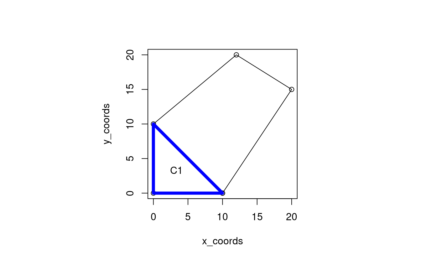

FIGURE 10.2: Illustration of polygon centroid calculation problem.

Step 3 is to find the area of each triangle, so a weighted mean accounting for the disproportionate impact of large triangles is accounted for. The formula to calculate the area of a triangle is as follows (Kaiser and Morin 1993):

\[ \frac{Ax ( B y − C y ) + B x ( C y − A y ) + C x ( A y − B y )} { 2 } \]

Where \(A\) to \(C\) are the triangle’s three points and \(x\) and \(y\) refer to the x and y dimensions. A translation of this formula into R code that works with the data in the matrix representation of a triangle T1 is as follows (the function abs() ensures a positive result):

# calculate the area of the triangle represented by matrix T1:
abs(T1[1, 1] * (T1[2, 2] - T1[3, 2]) +
  T1[2, 1] * (T1[3, 2] - T1[1, 2]) +
  T1[3, 1] * (T1[1, 2] - T1[2, 2]) ) / 2
#> [1] 50

This code chunk outputs the correct result.⁶¹ The problem is that code is clunky and must by re-typed if we want to run it on another triangle matrix. To make the code more generalizable, we will see how it can be converted into a function in Section 10.4.

Step 4 requires steps 2 and 3 to be undertaken not just on one triangle (as demonstrated above) but on all triangles. This requires iteration to create all triangles representing the polygon, illustrated in Figure 10.3. lapply() and vapply() are used to iterate over each triangle here because they provide a concise solution in base R:⁶²

i = 2:(nrow(poly_mat) - 2)
T_all = lapply(i, function(x) {
  rbind(Origin, poly_mat[x:(x + 1), ], Origin)
})

C_list = lapply(T_all,  function(x) (x[1, ] + x[2, ] + x[3, ]) / 3)
C = do.call(rbind, C_list)

A = vapply(T_all, function(x) {
  abs(x[1, 1] * (x[2, 2] - x[3, 2]) +
        x[2, 1] * (x[3, 2] - x[1, 2]) +
        x[3, 1] * (x[1, 2] - x[2, 2]) ) / 2
  }, FUN.VALUE = double(1))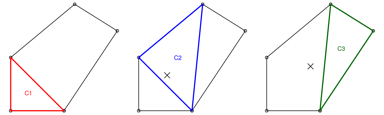

FIGURE 10.3: Illustration of iterative centroid algorithm with triangles. The X represents the area-weighted centroid in iterations 2 and 3.

We are now in a position to complete step 4 to calculate the total area with sum(A) and the centroid coordinates of the polygon with weighted.mean(C[, 1], A) and weighted.mean(C[, 2], A) (exercise for alert readers: verify these commands work). To demonstrate the link between algorithms and scripts, the contents of this section have been condensed into 10-centroid-alg.R. We saw at the end of Section 10.2 how this script can calculate the centroid of a square. The great thing about scripting the algorithm is that it works on the new poly_mat object (see exercises below to verify these results with reference to st_centroid()):

source("code/10-centroid-alg.R")
#> [1] "The area is: 245"
#> [1] "The coordinates of the centroid are: 8.83, 9.22"

The example above shows that low-level geographic operations can be developed from first principles with base R. It also shows that if a tried-and-tested solution already exists, it may not be worth re-inventing the wheel: if we aimed only to find the centroid of a polygon, it would have been quicker to represent poly_mat as an sf object and use the pre-existing sf::st_centroid() function instead. However, the great benefit of writing algorithms from 1^st principles is that you will understand every step of the process, something that cannot be guaranteed when using other peoples’ code. A further consideration is performance: R is slow compared with low-level languages such as C++ for number crunching (see Section 1.3) and optimization is difficult. If the aim is to develop new methods, computational efficiency should not be prioritized. This is captured in the saying “premature optimization is the root of all evil (or at least most of it) in programming” (Knuth 1974).

Algorithm development is hard. This should be apparent from the amount of work that has gone into developing a centroid algorithm in base R that is just one, rather inefficient, approach to the problem with limited real-world applications (convex polygons are uncommon in practice). The experience should lead to an appreciation of low-level geographic libraries such as GEOS (which underlies sf::st_centroid()) and CGAL (the Computational Geometry Algorithms Library) which not only run fast but work on a wide range of input geometry types. A great advantage of the open source nature of such libraries is that their source code is readily available for study, comprehension and (for those with the skills and confidence) modification.⁶³

10.4 Functions

Like algorithms, functions take an input and return an output. Functions, however, refer to the implementation in a particular programming language, rather than the ‘recipe’ itself. In R, functions are objects in their own right, that can be created and joined together in a modular fashion. We can, for example, create a function that undertakes step 2 of our centroid generation algorithm as follows:

t_centroid = function(x) {
  (x[1, ] + x[2, ] + x[3, ]) / 3
}

The above example demonstrates two key components of functions: 1) the function body, the code inside the curly brackets that define what the function does with the inputs; and 2) the formals, the list of arguments the function works with — x in this case (the third key component, the environment, is beyond the scope of this section). By default, functions return the last object that has been calculated (the coordinates of the centroid in the case of t_centroid()).⁶⁴

The function now works on any inputs you pass it, as illustrated in the below command which calculates the area of the 1^st triangle from the example polygon in the previous section (see Figure 10.3):

t_centroid(T1)
#> x_coords y_coords 
#>     3.33     3.33

We can also create a function to calculate a triangle’s area, which we will name t_area():

t_area = function(x) {
  abs(
    x[1, 1] * (x[2, 2] - x[3, 2]) +
    x[2, 1] * (x[3, 2] - x[1, 2]) +
    x[3, 1] * (x[1, 2] - x[2, 2])
  ) / 2
}

Note that after the function’s creation, a triangle’s area can be calculated in a single line of code, avoiding duplication of verbose code: functions are a mechanism for generalizing code. The newly created function t_area() takes any object x, assumed to have the same dimensions as the ‘triangle matrix’ data structure we’ve been using, and returns its area, as illustrated on T1 as follows:

t_area(T1)
#> [1] 50

We can test the generalizability of the function by using it to find the area of a new triangle matrix, which has a height of 1 and a base of 3:

t_new = cbind(x = c(0, 3, 3, 0),
              y = c(0, 0, 1, 0))
t_area(t_new)
#>   x 
#> 1.5

A useful feature of functions is that they are modular. Provided that you know what the output will be, one function can be used as the building block of another. Thus, the functions t_centroid() and t_area() can be used as sub-components of a larger function to do the work of the script 10-centroid-alg.R: calculate the area of any convex polygon. The code chunk below creates the function poly_centroid() to mimic the behavior of sf::st_centroid() for convex polygons:⁶⁵

poly_centroid = function(poly_mat) {
  Origin = poly_mat[1, ] # create a point representing the origin
  i = 2:(nrow(poly_mat) - 2)
  T_all = lapply(i, function(x) {
    rbind(Origin, poly_mat[x:(x + 1), ], Origin)
  })
  C_list = lapply(T_all, t_centroid)
  C = do.call(rbind, C_list)
  A = vapply(T_all, t_area, FUN.VALUE = double(1))
  c(weighted.mean(C[, 1], A), weighted.mean(C[, 2], A))
}

poly_centroid(poly_mat)
#> [1] 8.83 9.22

Functions such as poly_centroid() can further be extended to provide different types of output. To return the result as an object of class sfg, for example, a ‘wrapper’ function can be used to modify the output of poly_centroid() before returning the result:

poly_centroid_sfg = function(x) {
  centroid_coords = poly_centroid(x)
  sf::st_point(centroid_coords)
}

We can verify that the output is the same as the output from sf::st_centroid() as follows:

poly_sfc = sf::st_polygon(list(poly_mat))
identical(poly_centroid_sfg(poly_mat), sf::st_centroid(poly_sfc))
#> [1] TRUE

10.5 Programming

In this chapter we have moved quickly, from scripts to functions via the tricky topic of algorithms. Not only have we discussed them in the abstract, but we have also created working examples of each to solve a specific problem:

• The script 10-centroid-alg.R was introduced and demonstrated on a ‘polygon matrix’
• The individual steps that allowed this script to work were described as an algorithm, a computational recipe
• To generalize the algorithm we converted it into modular functions which were eventually combined to create the function poly_centroid() in the previous section

Taken on its own, each of these steps is straightforward. But the skill of programming is combining scripts, algorithms and functions in a way that produces performant, robust and user-friendly tools that other people can use. If you are new to programming, as we expect most people reading this book will be, being able to follow and reproduce the results in the preceding sections should be seen as a major achievement. Programming takes many hours of dedicated study and practice before you become proficient.

The challenge facing developers aiming to implement new algorithms in an efficient way is put in perspective by considering that we have only created a toy function. In its current state, poly_centroid() fails on most (non-convex) polygons! A question arising from this is: how would one generalize the function? Two options are (1) to find ways to triangulate non-convex polygons (a topic covered in the online algorithm article that supports this chapter) and (2) to explore other centroid algorithms that do not rely on triangular meshes.

A wider question is: is it worth programming a solution at all when high performance algorithms have already been implemented and packaged in functions such as st_centroid()? The reductionist answer in this specific case is ‘no.’ In the wider context, and considering the benefits of learning to program, the answer is ‘it depends.’ With programming, it’s easy to waste hours trying to implement a method, only to find that someone has already done the hard work. So instead of seeing this chapter as your first stepping stone towards geometric algorithm programming wizardry, it may be more productive to use it as a lesson in when to try to program a generalized solution, and when to use existing higher-level solutions. There will surely be occasions when writing new functions is the best way forward, but there will also be times when using functions that already exist is the best way forward.

We cannot guarantee that, having read this chapter, you will be able to rapidly create new functions for your work. But we are confident that its contents will help you decide when is an appropriate time to try (when no other existing functions solve the problem, when the programming task is within your capabilities and when the benefits of the solution are likely to outweigh the time costs of developing it). First steps towards programming can be slow (the exercises below should not be rushed) but the long-term rewards can be large.

10.6 Exercises

1. Read the script 10-centroid-alg.R in the code folder of the book’s GitHub repo.
   • Which of the best practices covered in Section 10.2 does it follow?
   • Create a version of the script on your computer in an IDE such as RStudio (preferably by typing-out the script line-by-line, in your own coding style and with your own comments, rather than copy-pasting — this will help you learn how to type scripts). Using the example of a square polygon (e.g., created with poly_mat = cbind(x = c(0, 0, 9, 9, 0), y = c(0, 9, 9, 0, 0))) execute the script line-by-line.
   • What changes could be made to the script to make it more reproducible?
   • How could the documentation be improved?
2. In Section 10.3 we calculated that the area and geographic centroid of the polygon represented by poly_mat was 245 and 8.8, 9.2, respectively.
   • Reproduce the results on your own computer with reference to the script 10-centroid-alg.R, an implementation of this algorithm (bonus: type out the commands - try to avoid copy-pasting).
   • Are the results correct? Verify them by converting poly_mat into an sfc object (named poly_sfc) with st_polygon() (hint: this function takes objects of class list()) and then using st_area() and st_centroid().
3. It was stated that the algorithm we created only works for convex hulls. Define convex hulls (see Chapter 5) and test the algorithm on a polygon that is not a convex hull.
   • Bonus 1: Think about why the method only works for convex hulls and note changes that would need to be made to the algorithm to make it work for other types of polygon.
   • Bonus 2: Building on the contents of 10-centroid-alg.R, write an algorithm only using base R functions that can find the total length of linestrings represented in matrix form.
4. In Section 10.4 we created different versions of the poly_centroid() function that generated outputs of class sfg (poly_centroid_sfg()) and type-stable matrix outputs (poly_centroid_type_stable()). Further extend the function by creating a version (e.g., called poly_centroid_sf()) that is type stable (only accepts inputs of class sf) and returns sf objects (hint: you may need to convert the object x into a matrix with the command sf::st_coordinates(x)).
   • Verify it works by running poly_centroid_sf(sf::st_sf(sf::st_sfc(poly_sfc)))
   • What error message do you get when you try to run poly_centroid_sf(poly_mat)?